please help me to solve these questions.

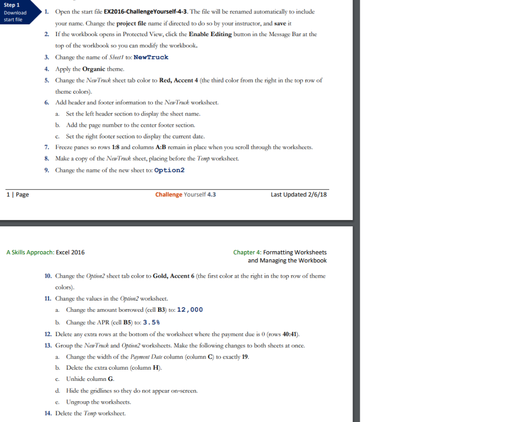
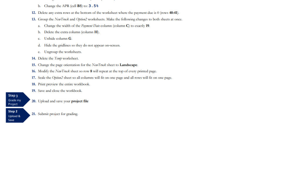
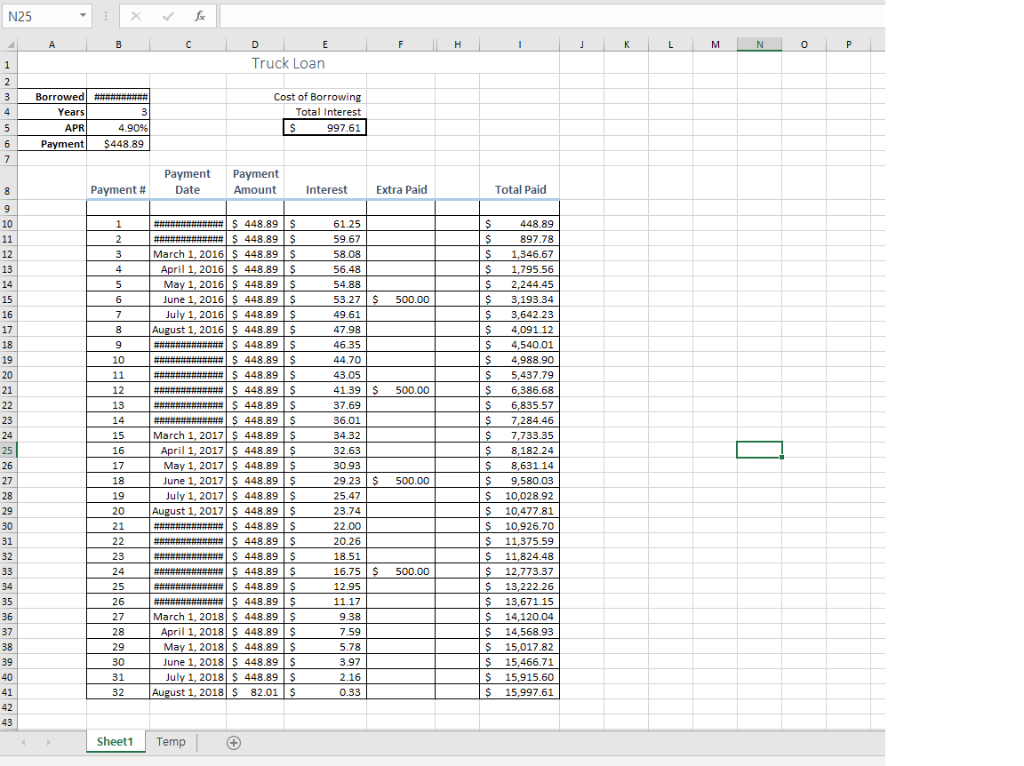
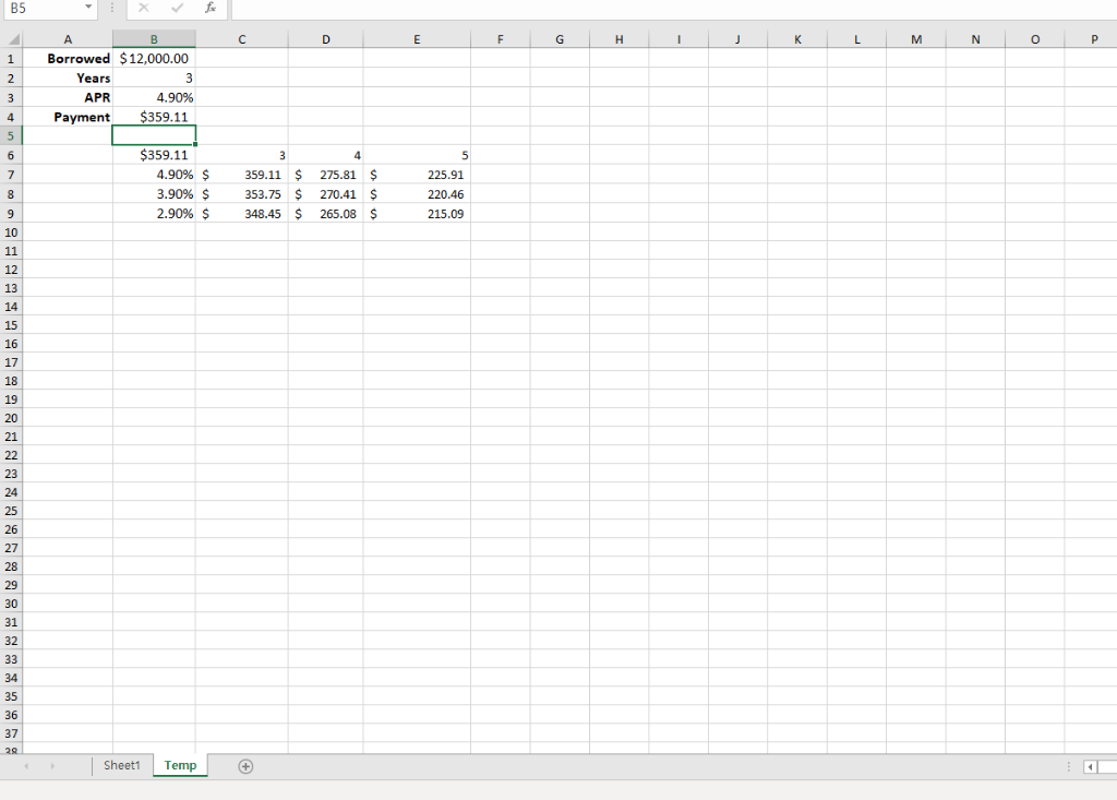
Step 1 Download start file 1. Open the start file EX2016-ChageYourself-4-3. The file will be renamed automatically to include your name. Change the project file name if directed to do so by your instructor, and save it 2. If the workbook opens in Protected View, click the Enable Editing button in the Message Bar at the top of the workbook so you can modify the workbook 3. Change the name of Sheetl to: NewTruck 4. Apply the Organic theme. 5. Change the NewTruck sheet tab color to Red, Accent 4 (the third color from the right in the top row of theme colors). 6. Add header and footer information to the New Truck worksheet. Set the left header section to display the sheet name. a. b. Add the page number to the center footer section. Set the right footer section to display the current date. Freeze panes so rows 1:8 and columns A:B remain in place when you scroll through the worksheets. Make a copy of the New Truck sheet, placing before the Temp worksheet. Change the name of the new sheet to: Option2 c. 7. 8. 9. 1| Page Last Updated 2/6/18 Challenge Yourself 4.3 A Skills Approach: Excel 2016 Chapter 4: Formatting Worksheets and Managing the Workbook 10. Change the Option2 sheet tab color to Gold, Accent 6 (the first color at the right in the top row of theme colors). 11. Change the values in the Option2 worksheet Change the amount borrowed (cell B3) to: 12, 000 a. b. Change the APR (cell B5) to: 3 . 5% 12. Delete any extra rows at the bottom of the worksheet where the payment due is 0 (rows 40:41 13. Group the Nea Truck and Option2 worksheets. Make the following changes to both sheets at once a. Change the width of the Payment Date column (column C) to exactly 19 b. Delete the extra column (column H). c. Unhide column G d. Hide the gridlines so they do not appear on-screen. e. Ungroup the worksheets. 14. Delete the Temp worksheet. b, Change the APR (cell B5) to: 3.5% 12. Delete any extra rows at the bottom of the worksheet where the payment due is O (rows 40:41 13. Group the New Truck and Option2 worksheets. Make the following changes to both sheets at once Change the width of the Payment Date column (column C) to exactly 19 a. b. Delete the extra column (column H) Unhide column G. c. d. Hide the gridlines so they do not appear on-screen Ungroup the worksheets 14. Delete the Temp worksheet. 15. Change the page orientation for the NewTruok sheet to Landscape. 16. Modify the Nea Truck sheet 7. Scale the Option2 sheet so all columns will fit on one page and all rows will fit on one page. 18. Print preview the entire workbook. 19. Save and close the workbook so row 8 will repeat at the top of every printed page. Step 3 Grade my 20. Upload and save your project file Step 2 Upload & Save 21. Submit project for grading N25 Truck Loan Cost of Borrowing Total Interest 997.61 Years APR 4.90% 448.89 Payment Payment Payment # Date Amount Interest Extra Paid Total Paid 61.25 59.67 58.08 56.48 54.88 53.27 49.61 47.98 46.35 44.70 448.89 897.78 1,346.67 1,795.56 2,244.45 ,193.34 3,642.23 4,091.12 4,540.01 4,988.9 5,437.79 6,386.68 6.835.57 7.284.46 7,733.35 8,182.24 8,631.14 $ 9,580.03 March 1, 2016 S 448.89 il 1, 2016 $ 448.89 2016 S 448.89 June 1, 2016 $ 448.89 July 1, 2016$448.89 August 1, 2016 $ 448.89 500.00 448.89 448.89 448.89 41.39 37.69 36.01 34.32 32.63 30.93 500.00 March 1, 2017 448.89 ril 1, 2017 $ 448.89 May 1, 2017 S 448.89 June 1, 2017 448.89 $ 500.00 July 1, 2017 448.89 August 1, 2017 $ 448.89 23.74 22.00 0.26 18.51 16.75 12.95 10,477.81 10 926.70 11,375.59 11,824.48 12,773.37 13,222.26 13,671.15 14,120.04 14,568.93 448.89 448.89 448.89 500.00 27 March 1, 2018 S 448.89 S April 1. 2018 S 448,89 May 1, 2018 5 448.89 June 1, 2018 448.89 July 1, 2018 $ 448.89 9.38 15,466.71 15,915.60 15,997.61 5 August 1, 2018 82.01 SheeTemp B5 1 Borrowed $12,000.00 Years 4.90% Payment $359.11 $359.11 APR 225.91 220.46 215.09 4.90% $ 359.11 $ 275.81 $ 3.90% $ 353.75 $ 270.41 $ 2.90% $ 348.45 $ 265.08 $ 10 12 14 15 16 17 18 19 25 29 31 32 35 37 SheetTemp Step 1 Download start file 1. Open the start file EX2016-ChageYourself-4-3. The file will be renamed automatically to include your name. Change the project file name if directed to do so by your instructor, and save it 2. If the workbook opens in Protected View, click the Enable Editing button in the Message Bar at the top of the workbook so you can modify the workbook 3. Change the name of Sheetl to: NewTruck 4. Apply the Organic theme. 5. Change the NewTruck sheet tab color to Red, Accent 4 (the third color from the right in the top row of theme colors). 6. Add header and footer information to the New Truck worksheet. Set the left header section to display the sheet name. a. b. Add the page number to the center footer section. Set the right footer section to display the current date. Freeze panes so rows 1:8 and columns A:B remain in place when you scroll through the worksheets. Make a copy of the New Truck sheet, placing before the Temp worksheet. Change the name of the new sheet to: Option2 c. 7. 8. 9. 1| Page Last Updated 2/6/18 Challenge Yourself 4.3 A Skills Approach: Excel 2016 Chapter 4: Formatting Worksheets and Managing the Workbook 10. Change the Option2 sheet tab color to Gold, Accent 6 (the first color at the right in the top row of theme colors). 11. Change the values in the Option2 worksheet Change the amount borrowed (cell B3) to: 12, 000 a. b. Change the APR (cell B5) to: 3 . 5% 12. Delete any extra rows at the bottom of the worksheet where the payment due is 0 (rows 40:41 13. Group the Nea Truck and Option2 worksheets. Make the following changes to both sheets at once a. Change the width of the Payment Date column (column C) to exactly 19 b. Delete the extra column (column H). c. Unhide column G d. Hide the gridlines so they do not appear on-screen. e. Ungroup the worksheets. 14. Delete the Temp worksheet. b, Change the APR (cell B5) to: 3.5% 12. Delete any extra rows at the bottom of the worksheet where the payment due is O (rows 40:41 13. Group the New Truck and Option2 worksheets. Make the following changes to both sheets at once Change the width of the Payment Date column (column C) to exactly 19 a. b. Delete the extra column (column H) Unhide column G. c. d. Hide the gridlines so they do not appear on-screen Ungroup the worksheets 14. Delete the Temp worksheet. 15. Change the page orientation for the NewTruok sheet to Landscape. 16. Modify the Nea Truck sheet 7. Scale the Option2 sheet so all columns will fit on one page and all rows will fit on one page. 18. Print preview the entire workbook. 19. Save and close the workbook so row 8 will repeat at the top of every printed page. Step 3 Grade my 20. Upload and save your project file Step 2 Upload & Save 21. Submit project for grading N25 Truck Loan Cost of Borrowing Total Interest 997.61 Years APR 4.90% 448.89 Payment Payment Payment # Date Amount Interest Extra Paid Total Paid 61.25 59.67 58.08 56.48 54.88 53.27 49.61 47.98 46.35 44.70 448.89 897.78 1,346.67 1,795.56 2,244.45 ,193.34 3,642.23 4,091.12 4,540.01 4,988.9 5,437.79 6,386.68 6.835.57 7.284.46 7,733.35 8,182.24 8,631.14 $ 9,580.03 March 1, 2016 S 448.89 il 1, 2016 $ 448.89 2016 S 448.89 June 1, 2016 $ 448.89 July 1, 2016$448.89 August 1, 2016 $ 448.89 500.00 448.89 448.89 448.89 41.39 37.69 36.01 34.32 32.63 30.93 500.00 March 1, 2017 448.89 ril 1, 2017 $ 448.89 May 1, 2017 S 448.89 June 1, 2017 448.89 $ 500.00 July 1, 2017 448.89 August 1, 2017 $ 448.89 23.74 22.00 0.26 18.51 16.75 12.95 10,477.81 10 926.70 11,375.59 11,824.48 12,773.37 13,222.26 13,671.15 14,120.04 14,568.93 448.89 448.89 448.89 500.00 27 March 1, 2018 S 448.89 S April 1. 2018 S 448,89 May 1, 2018 5 448.89 June 1, 2018 448.89 July 1, 2018 $ 448.89 9.38 15,466.71 15,915.60 15,997.61 5 August 1, 2018 82.01 SheeTemp B5 1 Borrowed $12,000.00 Years 4.90% Payment $359.11 $359.11 APR 225.91 220.46 215.09 4.90% $ 359.11 $ 275.81 $ 3.90% $ 353.75 $ 270.41 $ 2.90% $ 348.45 $ 265.08 $ 10 12 14 15 16 17 18 19 25 29 31 32 35 37 SheetTemp