please help me with mathlab


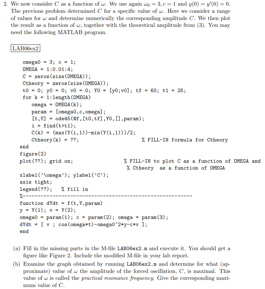
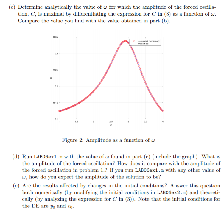
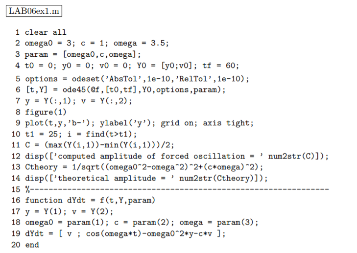
2. We now consider C as a function of w. We use again wo 3, c 1 and y(0) y(0-0 The previous problem determined C for a specific value of w. Here we consider a range of values for w and determine numerically the corresponding amplitude C. We then plot the result as a function of w, together with the theoretical amplitude from (3). You may need the following MATLAB progranm LAB06ex2 omega0 3; c-1; OMEGA1:0.01:4; C- zeros (size(OMEGA)); Ctheory -zeros (size (OMEGA)) for k -1:length (OMEGA) omega - 0MEGA (k); param - [omega0,c, omega]; [t,Y] = ode45 (Qf, [t0 ,tf],YO ,[],param); i-find (t>t1); C(k) (max(y(i,1))-min (Y (i ,1)))/2; Ctheory (k) ?? ; % FILL-IN formula for Ctheory figure (2) plot(??); grid on; % FILL-IN to plot C as a function of OMEGA and % Ctheory as a function of OMEGA xlabel('omega) ylabel('C') axis tight; legend(7?); % fill in function dYdt f(t,Y,param) = omega0 param(1); c - param (2); omega -param (3); end (a) Fill in the missing parts in the M-file LAB06ex2.m and execute it. You should get a figure like Figure 2. Include the modified M-file in your lab report (b) Examine the graph obtained by running LAB06ex2.m and determine for what (ap proximate) value of w the amplitude of the forced oscillation, C, is maximal. This value of w is called the practical resonance frequency. Give the corresponding maxi- mum value of C. 2. We now consider C as a function of w. We use again wo 3, c 1 and y(0) y(0-0 The previous problem determined C for a specific value of w. Here we consider a range of values for w and determine numerically the corresponding amplitude C. We then plot the result as a function of w, together with the theoretical amplitude from (3). You may need the following MATLAB progranm LAB06ex2 omega0 3; c-1; OMEGA1:0.01:4; C- zeros (size(OMEGA)); Ctheory -zeros (size (OMEGA)) for k -1:length (OMEGA) omega - 0MEGA (k); param - [omega0,c, omega]; [t,Y] = ode45 (Qf, [t0 ,tf],YO ,[],param); i-find (t>t1); C(k) (max(y(i,1))-min (Y (i ,1)))/2; Ctheory (k) ?? ; % FILL-IN formula for Ctheory figure (2) plot(??); grid on; % FILL-IN to plot C as a function of OMEGA and % Ctheory as a function of OMEGA xlabel('omega) ylabel('C') axis tight; legend(7?); % fill in function dYdt f(t,Y,param) = omega0 param(1); c - param (2); omega -param (3); end (a) Fill in the missing parts in the M-file LAB06ex2.m and execute it. You should get a figure like Figure 2. Include the modified M-file in your lab report (b) Examine the graph obtained by running LAB06ex2.m and determine for what (ap proximate) value of w the amplitude of the forced oscillation, C, is maximal. This value of w is called the practical resonance frequency. Give the corresponding maxi- mum value of C
