please I want the answers with explanation

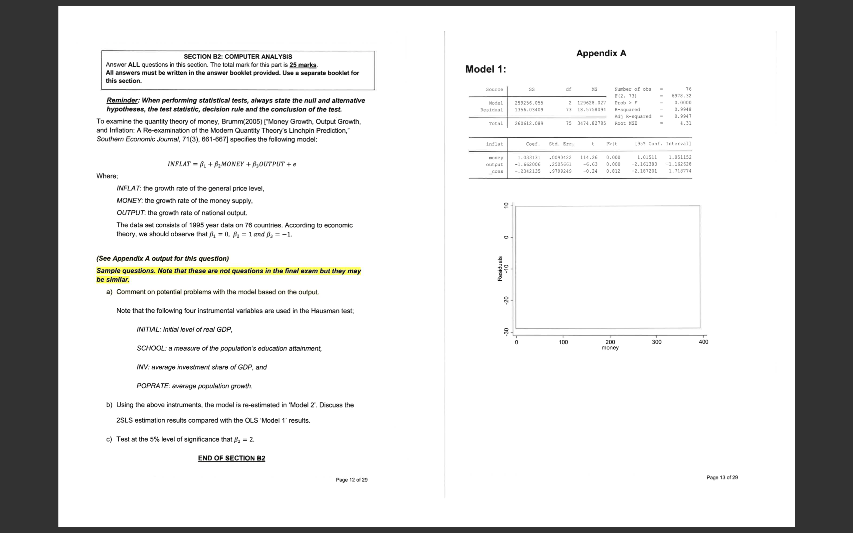
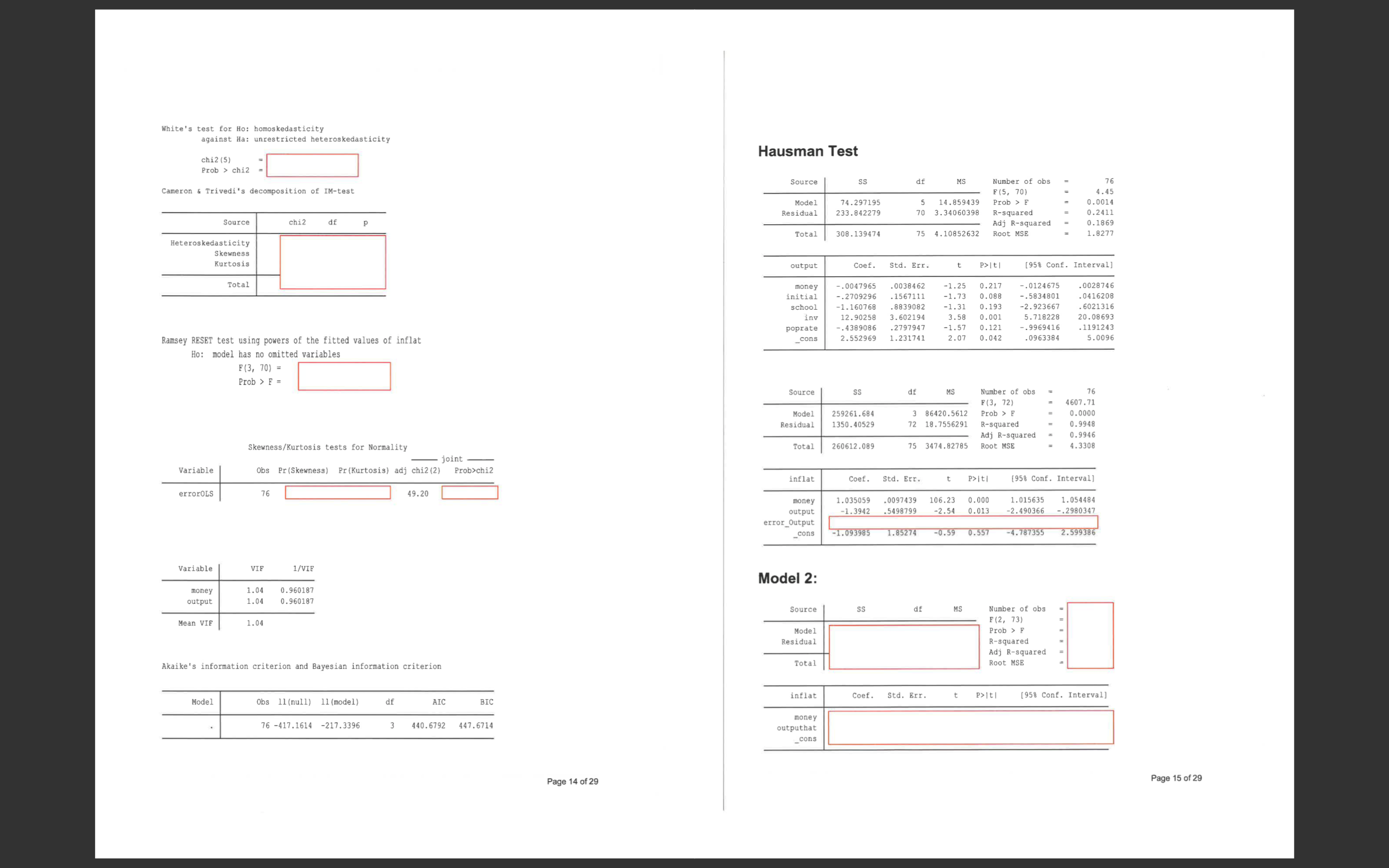
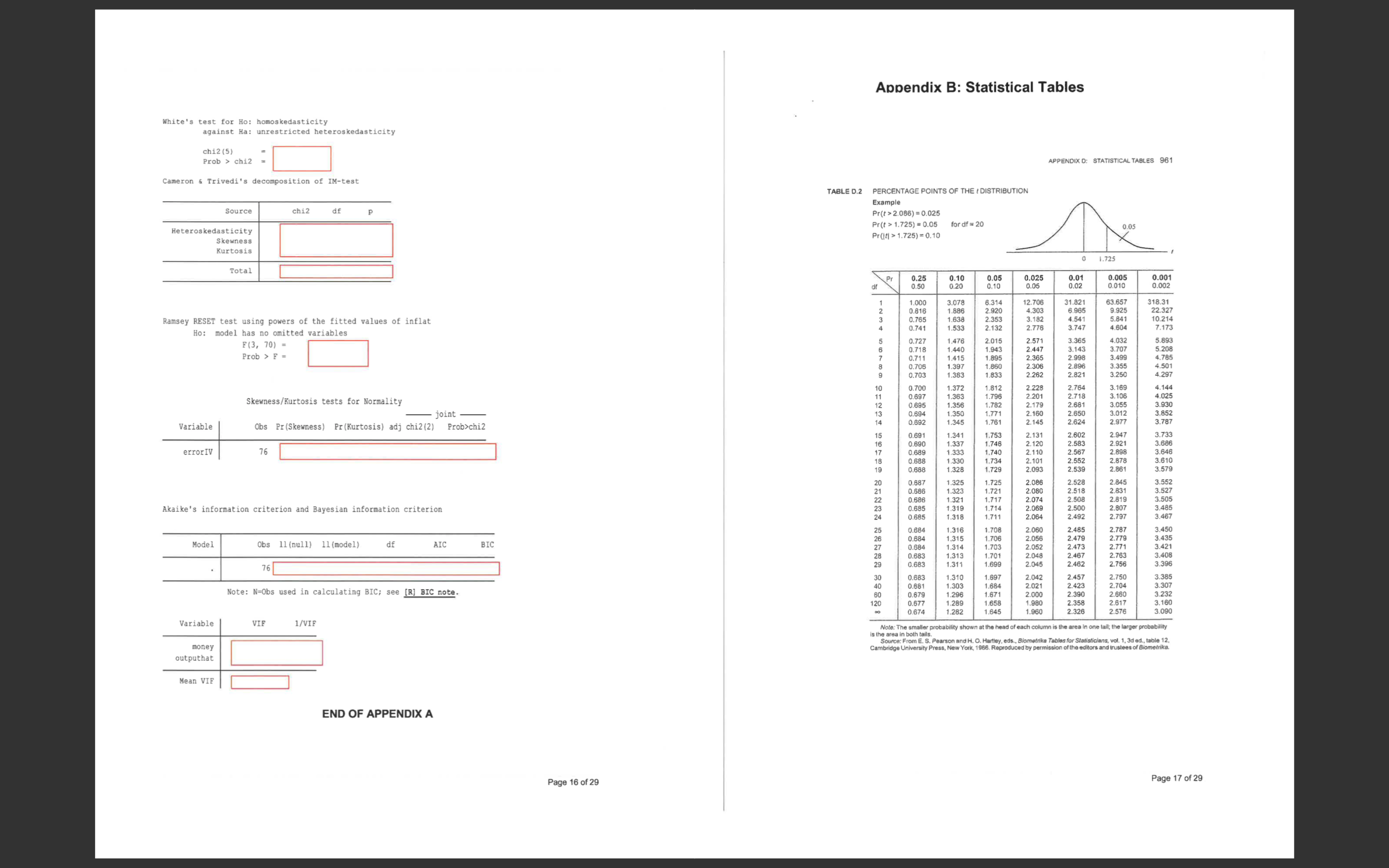
SECTION B2: COMPUTER ANALYSIS Appendix A Answer ALL questions in this section. The total mark for this part is 25 marks. All answers must be written in the answer booklet provided. Use a separate booklet for Model 1: this section. Source df MS Number of obs 76 Reminder: When performing statistical tests, always state the null and alternative F (2, 73) 6978 .32 Model 259256.055 2 129628. 027 Prob > F 0. 0000 hypotheses, the test statistic, decision rule and the conclusion of the test Residual 1356.03409 3 18.5758094 R-squared 0. 9948 0. 9947 To examine the quantity theory of money, Brumm(2005) ["Money Growth, Output Growth, Adj R-squared Total 260612.089 75 3474.82785 Root MSE 4.31 and Inflation: A Re-examination of the Modern Quantity Theory's Linchpin Prediction," Southern Economic Journal, 71(3), 661-667] specifies the following model: inflat Coef. Std. Err. P>It| [958 Conf. Interval] 1. 033131 . 0090422 114.26 0. 000 1. 01511 1. 051152 INFLAT = B1 + 2MONEY + B3OUTPUT + e money output -1. 662006 .2505661 -6.63 0. 000 -2. 161383 -1. 162628 _cons -.2342135 . 9799249 0.24 0. 812 -2. 187201 1. 718774 Where; INFLAT: the growth rate of the general price level, MONEY: the growth rate of the money supply, 2 - OUTPUT: the growth rate of national output. The data set consists of 1995 year data on 76 countries. According to economic theory, we should observe that B1 = 0, B2 = 1 and B3 = -1. (See Appendix A output for this question) Sample questions. Note that these are not questions in the final exam but they may be similar. Residuals -10 a) Comment on potential problems with the model based on the output. -20 Note that the following four instrumental variables are used in the Hausman test; INITIAL: Initial level of real GDP, -30 10 200 300 400 SCHOOL: a measure of the population's education attainment, money INV: average investment share of GDP, and POPRATE: average population growth. b) Using the above instruments, the model is re-estimated in 'Model 2'. Discuss the 2SLS estimation results compared with the OLS 'Model 1' results. c) Test at the 5% level of significance that B2 = 2. END OF SECTION B2 Page 12 of 29 Page 13 of 29White's test for Ho: homoskedasticity against Ha: unrestricted heteroskedasticity chi2 (5) Hausman Test Prob > chi2 Cameron & Trivedi's decomposition of IM-test Source SS df MS Number of obs 76 F (5, 70) 4.45 Model 74.297195 . 0014 Source chi2 df P Residual 233.842279 5 14.859439 70 3.34060398 Prob > R-squared 0.2411 Adj R-squared .1869 Heteroskedasticity Total 308 .139474 4.10852632 Root MSE 1.8277 Skewness Kurtosis output Coef. Std. Err. P>Iti [958 Conf. Interval] Total money . 0047965 . 0038462 -1.25 . 0028746 nitial . 2709296 0.217 . 1567111 - . 0124675 0. 088 -1. 160768 -. 5834801 . 0416208 school . 8839082 -1. 13 -1.31 0. 193 inv 12. 90258 3. 602194 3.58 0.001 -2. 923667 6021316 Ramsey RESET test using powers of the fitted values of inflat oprate . 4389086 .2797947 20. 08693 -1.57 5. 718228 0. 121 . 1191243 _cons 2.552969 1.231741 2.07 0. 042 -. 9969416 . 0963384 5.0096 Ho: model has no omitted variables F (3, 70) = Prob > F = Source SS df MS Number of obs 76 F (3, 72 4607.71 Model Residual 259261.684 0.000 1350. 40529 3 86420.5612 Prob > F 18 .7556291 R-squared 0. 9948 Skewness/Kurtosis tests for Normality Adj R-squared 0.9946 Total - joint - 260612.089 75 3474.82785 Root MSE 4. 3308 Variable Obs Pr (Skewness) Pr (Kurtosis) adj chi2 (2) Prob>chi2 inflat Coef. Std. Err. P>It/ [958 Conf. Interval] errorOLS 76 49.20 money 1.035059 . 0097439 106.23 0.000 output -1.3942 .5498799 -2.54 0. 013 1. 015635 2. 490366 1. 054484 -.2980347 error_Output _cons -1.093985 1. 85274 -0.59 0.557 -4.787355 2.599386 Variable VIF 1/VIF money 1.04 0. 960187 Model 2: output 1.04 0. 960187 Source SS df MS Mean VIE Number of obs 1.04 F (2, 73 Model Residual Prob > F R-squared Akaike's information criterion and Bayesian information criterion Adj R-squared Total Root MSE Model Obs 11 (null) 11 (model) df AIC BIC inflat Coef. Std. Err. t P>It| [958 Conf. Interval] 76 -417.1614 -217.3396 3 440. 6792 447. 6714 money outputhat _cons Page 14 of 29 Page 15 of 29Appendix B: Statistical Tables White's test for Ho: homoskedasticity against Ha: unrestricted heteroskedasticity chi2 (5) Prob > chi2 = APPENDIX D: STATISTICAL TABLES 961 Cameron & Trivedi's decomposition of IM-test TABLE D.2 PERCENTAGE POINTS OF THE ( DISTRIBUTION Source Example chi2 df Pr(t > 2.086) = 0.025 Heteroskedasticity Pr (t > 1.725) = 0.05 for df = 20 Pr(1{{ > 1.725) = 0.10 0.05 Skewness Kurtosis 1.725 Total 0.20 0.05 0.025 0.010 0.002 1.000 8.314 31.821 9.925 318.31 22.327 Ramsey RESET test using powers of the fitted values of inflat 2.353 4.303 3.182 4.541 5.841 10.214 Ho: model has no omitted variables 1.533 2.132 2.776 3.747 4 604 7.173 F (3, 70) = 0.727 2.015 2.571 3.365 4.032 5.893 Prob > F = 0.718 1.440 3.143 3.707 2.998 0.703 1.383 1.833 2.262 2.896 2.821 3.355 3.250 1.812 2.764 Skewness/Kurtosis tests for Normality 2.718 Variable 83828 88888 1.372 3.169 3.106 4.144 4.025 joint 1:771 Obs Pr(Skewness) Pr(Kurtosis) adj chi2 (2) Prob>chi2 1.781 2. 145 2.650 2.624 3.852 3.787 2.131 error IV 76 2. 120 2.602 2.583 2.947 3.733 2.567 2.921 2.101 2.093 2.539 2.878 2.861 3.579 0.687 2.086 2.528 2.845 3.552 2-631 Akaike's information criterion and Bayesian information criterion 0. 685 2.064 2.500 2.492 2.797 3.467 2.787 3.450 Model Obs 11 (null) 11 (model) df AIC BIC 2.479 2.779 2.048 2.473 2.467 2.771 3.435 2.763 76 89888 2.045 2.462 2.756 0.68 Note: N=Obs used in calculating BIC; see [R] BIC note. 0.68 1.310 1.303 THE 82828 8 8 2.042 2.021 2.457 2.750 2 680 3:307 0.677 2 .358 2.617 3. 232 2.576 3.160 Variable VIE 1/VIF Note: The smaller probabili money Source: From E. S. Per Cambridge University Press, New York, 1966. R outputhat Mean VIE END OF APPENDIX A Page 16 of 29 Page 17 of 29