Please Interpret all results using the formula provided. Explain the results of P, t and standard error, Coefficients and R-Squared and overall significance of the regression.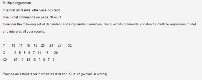

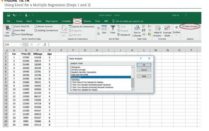
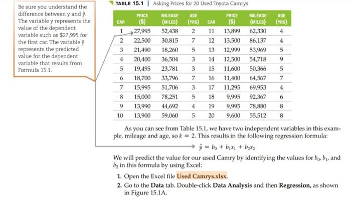
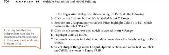
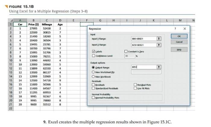
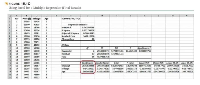
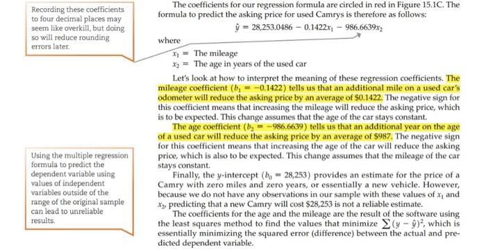
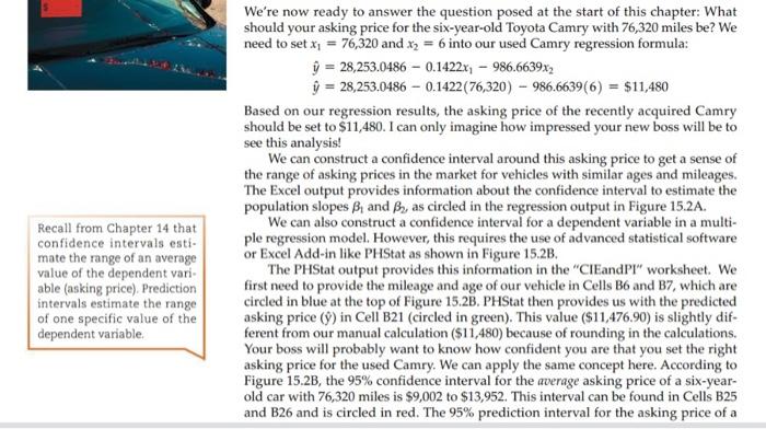
Please also explain in words for the estimate value on Y when x1=10 and x2=12

Multiple regression Interpret all results, otherwise no credit. Use Excel commands on page 703-704 Consider the following set of dependent and independent variables. Using excel commands, construct a multiple regression model and interpret all your results: Y 10 11 15 15 20 24 27 32 X1 2 5 5 9 7 11 16 20 X2 16 10 13 10 2 874 Provide an estimate for Y when X1 =10 and X2 = 12 (explain in words). Using Excel for a Multiple Regression (Steps 1 and 2) File Home Insert Draw Page Layout Formulas Duta Review From Tex/CSV Recent Sources Queries & Connections From Web Existing Connections From Table/Range Properties Refresh All-Eat Links Get & Transform Data E A B D E Car Price (5) Mileage Age 1 2 27995 52438 22500 30815 2 3 21490 18260 20400 36504 19495 23781 18700 33796 15995 51705 15000 78251 13990 44692 13900 59060 13899 62330 13500 86137 12999 53969 12500 54718 11600 50366 11400 64567 11295 69953 92367 9995 9995 78880 9600 55512 Get Data 524 1 Nims 2 3 4 4567 567892=2XHIBAGN MORHAA8 10 11 12 13 14 15 16 17 18 19 20 21 7 9 10 11 12 13 14 15 16 17 18 19 20 7 5 3 3 7 3 5 4 5 4 4 5 9 5 7 4 6 8 8 Used Camrys IMP View Sort Excel Tell me what you want to do Clear Reapply Advanced Text to Columns Filter Sort & Fiber Queries & Connections F G H Data Analysis Analysis Tools Histogram Moving Average Random Number Generation Rank and Percentile Bagression Sampling t-Test Paired Two Sample for Mean t-Test Two-Sample Assuming Equal variances 1-Test Two-Sample Assuming Unequal Variances Test Two Sample for Means Data Tools L 7 OK Cancel Help Sign in What-If Forecast Outline Analysis Sheet Forecast O M N Data Analysis Analysis P Be sure you understand the difference between y and 9. The variable y represents the value of the dependent variable such as $27,995 for the first car. The variable y represents the predicted value for the dependent variable that results from Formula 15.1. TABLE 15.1 Asking Prices for 20 Used Toyota Camrys MILEAGE AGE PRICE MILEAGE AGE PRICE ($) CAR (MILES) (YRS) CAR ($) (MILES) (YRS) 1 27,995 52,438 2 11 13,899 62,330 4 2 22,500 30,815 7 12 13,500 86,137 4 3 21,490 18,260 5 13 12,999 3 14 12,500 53,969 5 54,718 9 4 20,400 36,504 5 19,495 15 11,600 50,366 5 6 18,700 11,400 64,567 7 7 15,995 23,781 3 33,796 7 16 51,706 3 17 78,251 5 18 44,692 4 19 4 8 15,000 11,295 69,953 9,995 92,367 9,995 6 9 13,990 78,880 8 10 13,900 59,060 5 20 9,600 55,512 8 As you can see from Table 15.1, we have two independent variables in this exam- ple, mileage and age, so k = 2. This results in the following regression formula: = bo + bx + bx We will predict the value for our used Camry by identifying the values for bo, by, and b in this formula by using Excel: 1. Open the Excel file Used Camrys.xlsx. 2. Go to the Data tab. Double-click Data Analysis and then Regression, as shown in Figure 15.1A. 704 CHAPTER 15 Multiple Regression and Model Building Excel requires that the independent variables be located in adjacent columns in the spreadsheet as shown in Figure 15.18. In the Regression dialog box, shown in Figure 15.1B, do the following: 3. Click on the first text box, which is labeled Input Y Range. 4. Because our y (dependent) variable is Price, highlight Cells B1 to B21, which includes the label "Price." 5. Click on the second text box, which is labeled Input X Range. 6. Highlight Cells C1 to D21. 7. Because labels were included in our data range, check the Labels, as Figure 15.1B shows. 8. Select Output Range in the Output Options section, and in the text box, click on Cell F1, as shown in Figure 15.1B. FIGURE 15.1B Using Excel for a Multiple Regression (Steps 3-8) A B C D E F 1 Car Price (S) Age Mileage 52438 2 1 27995 2 2 22500 30815 7 3 21490 18260 5 20400 36504 3 19495 23781 3 33796 7 18700 15995 15000 78251 51706 3 5 13990 44692 4 13900 59060 5 13899 62330 4 13500 86137 4 12999 53969 5 12500 54718 9 11600 50366 5 Besiduals Standardized Residuals Residual Plots Line Fit Plots 7 11400 64567 69953 4 11295 9995 92367 6 Normal Probability Plots 9995 78880 8 9600 55512 8 9. Excel creates the multiple regression results shown in Figure 15.1C. 3 4 5 6 7 8 9 10 11 12 13 14 15 16 17 18 19 20 21 22 45 6 TBSAHHAHAR 7 8 9 10 11 12 13 14 15 16 17 18 19 20 G Regression Input Input y Range: Input X Range: H Labels Confidence Level: Output options Qutput Range: O New Worksheet gly O New Workbook Residuals Normal Probability 5851:58521 SCS1:50521 Constant is zero SFS1 M ? X OK Cancel Help N FIGURE 15.1C Using Excel for a Multiple Regression (Final Result) A A 8 E F D Age 1 Car Price (5) Mileage SUMMARY OUTPUT 2 1 27995 52438 2 3 2 22500 30815 7 4 3 21490 5 Multiple R 5 4 R Square 6 5 Adjusted R Square 18260 20400 36504 3 19495 23781 3 18700 33796 15995 51706 15000 78251 7 Standard Error 7 3 8 7 Observations 9 8 5 10 9 4 ANOVA 13990 44692 13900 59060 11 10 5 12 11 13899 62330 4 Regression 13 Residual 14 13 Total 15 12 13500 86137 4 12999 53969 5 12500 54718 9 11600 50366 11400 64567 14 16 15 17 16 5 7 4 6 Intercept Mileage 10 17 11295 69953 19 18 9995 92367 Age 20 19 9995 78880 B 21 20 9600 55512 8 G Regression Statistics I K M N 0.743504968 0.552799638 0.50018783 3489.12908 20 of $$ MS Significance F 2 255828307.3 127914153.6 10.5071402 0.001069715 206958369.5 12174021.74 17 19 462786676.8 17702 21997.32695 34508,7702 Coefficients Stonderd Error Stot P-value Lower 95% Upper 95% Lower 95.0% Upper 95.0% 28253.04858 2965.056136 9.528672402 3.1269E-08 21997.32695 -0.14224537 0.040173013 -3.54081908 0.00251158 -0.22700302 -0.05748772 -0.22700302 -0.05748772 986.663882 418.0286589 2.36027808 0.03047345 -1868.62726 104.700505 -1868.62726-104.700505 H Recording these coefficients to four decimal places may seem like overkill, but doing so will reduce rounding errors later. Using the multiple regression formula to predict the dependent variable using values of independent variables outside of the range of the original sample can lead to unreliable results. The coefficients for our regression formula are circled in red in Figure 15.1C. The formula to predict the asking price for used Camrys is therefore as follows: = 28,253.0486 -0.1422x - 986.6639x2 where x = The mileage x= The age in years of the used car Let's look at how to interpret the meaning of these regression coefficients. The mileage coefficient (b = -0.1422) tells us that an additional mile on a used car's odometer will reduce the asking price by an average of $0.1422. The negative sign for this coefficient means that increasing the mileage will reduce the asking price, which is to be expected. This change assumes that the age of the car stays constant. The age coefficient (b-986.6639) tells us that an additional year on the age of a used car will reduce the asking price by an average of $987. The negative sign for this coefficient means that increasing the age of the car will reduce the asking price, which is also to be expected. This change assumes that the mileage of the car stays constant. Finally, the y-intercept (b, 28,253) provides an estimate for the price of a Camry with zero miles and zero years, or essentially a new vehicle. However, because we do not have any observations in our sample with these values of x, and x, predicting that a new Camry will cost $28,253 is not a reliable estimate. The coefficients for the age and the mileage are the result of the software using the least squares method to find the values that minimize (y-), which is essentially minimizing the squared error (difference) between the actual and pre- dicted dependent variable. Recall from Chapter 14 that confidence intervals esti- mate the range of an average value of the dependent vari- able (asking price). Prediction intervals estimate the range of one specific value of the dependent variable. We're now ready to answer the question posed at the start of this chapter: What should your asking price for the six-year-old Toyota Camry with 76,320 miles be? We need to set x = 76,320 and x = 6 into our used Camry regression formula: 28,253.0486 0.1422x - 986.6639x2 = 28,253.0486 -0.1422 (76,320) 986.6639(6) = $11,480 Based on our regression results, the asking price of the recently acquired Camry should be set to $11,480. I can only imagine how impressed your new boss will be to see this analysis! We can construct a confidence interval around this asking price to get a sense of the range of asking prices in the market for vehicles with similar ages and mileages. The Excel output provides information about the confidence interval to estimate the population slopes B, and B, as circled in the regression output in Figure 15.2A. We can also construct a confidence interval for a dependent variable in a multi- ple regression model. However, this requires the use of advanced statistical software or Excel Add-in like PHStat as shown in Figure 15.2B. The PHStat output provides this information in the "CIEandPI" worksheet. We first need to provide the mileage and age of our vehicle in Cells B6 and B7, which are circled in blue at the top of Figure 15.2B. PHStat then provides us with the predicted asking price (y) in Cell B21 (circled in green). This value ($11,476.90) is slightly dif- ferent from our manual calculation ($11,480) because of rounding in the calculations. Your boss will probably want to know how confident you are that you set the right asking price for the used Camry. We can apply the same concept here. According to Figure 15.2B, the 95% confidence interval for the average asking price of a six-year- old car with 76,320 miles is $9,002 to $13,952. This interval can be found in Cells B25 and B26 and is circled in red. The 95% prediction interval for the asking price of a