please make sure to answer correctly in the problems of the excel, many other ones on chegg are incorrect and confusing. I will not hesitate to give a thumbs down if this is wrong. thank you in advance.

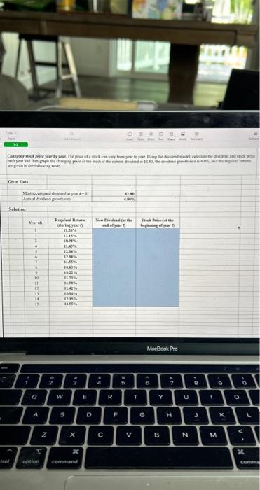
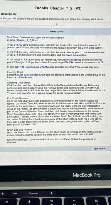
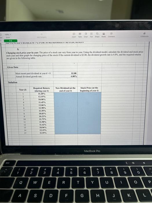
it fvenis be follewer uble. Description: oblem, you wal calculate the annual dividend and stock price and graph the changing stock prices. . Instructions Start Excel. Dewnload and open the workbock named: Brooks_Chapter 72 Start. In cel E14, by using cell references, calculate the dividend for year 1, Use the rumber of years in cell C14 and absplule references to the relevant cells from the Given Data section. In cell F14, by using cell references, calculate the stock price for year 1 . Use the new dividend in cell E14 and the relevant cells from the table and the Given Data secticn. In cell range E15:F28, by using cell references, calculate the dividends and stock prices for years 2 through 15. Copy the contents from cell range E14:F14 dewn the columns to row 28 . In celts C31:F45, insert a Line with Markers Chart for the Stock Price versus Year data. Inserting Chart Select the Line with Markers Chart from the provided chart options in the Charts group of the Insert tab of the Ribbon. Selecting Data Series Click the chart and then choose Select Data in the Design tab on the Rubbon. Delete any series created automatically using the Remove bution and add new series using the Add button. Select cells F14:F28 as the data range. Note that the Stock. Prices should stand for the Y values and Years for the X values. Leave the series name as Series1. Edit Chart Elements Go to the Add Chart Elements dropdown list in the Design tab of the Ribben. Delete the legend. Go to Axis Titles. Add Year as the tite for the horizontal axis. Next add Steck Price as the tite for the vertical axis. Next click anywhere in the Chart. Go to the Current Selecticn group of the Focthat tab of the Ribbon. Select Chart.Area in the dropdown list in the upper-left part of the Current Selection Group and then click. Formal Selection below. In the Format Chart Area dialog box, click Fal 8 Line option, then click Border group sign and select Solit Line option. Then go to the Color opton and select Black, Text 1. Go to top of the Gialog bex and select Plot Area from the dropdown menu of the Chart Options. Click Fl \& Line option. then dick Border group sign and select Solid Line. Neat change the color option to White, Eackground 1, Darker 15%. Chart Size and Position Go to the Fermat tab on the Roben. Set the chart height to 4 inches and the chart width to 7 inches. Drag the chart to position the entire char so that it fits within cells C31:F46. Save the workbook. Close the workbook and then exit Excel. Submit the workbock as directed. Changing stock price year by year. The price of a sock can vary froen year to year. Using the Evidend model, calculate the dividend and sock price Cach year and then griph the ckanging price of the stock if the curtent dvidend is $2.80, the dividend growth rate is 4 , OF5, and the required retums are given is the followin: table Given Data Most recent paid divident at year t=0 Antual dividend growth rale 5294.00% Solution MocBook Pre