Please Make sure to do it on Excel with Formula included

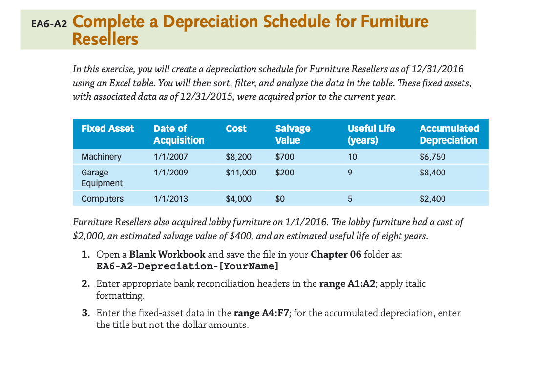
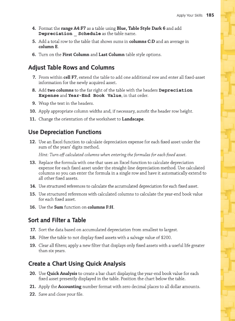
EA6-A2 Complete a Depreciation Schedule for Furniture Resellers In this exercise, you will create a depreciation schedule for Furniture Resellers as of 12/31/2016 using an Excel table. You will then sort, filter, and analyze the data in the table. These fixed assets, with associated data as of 12/31/2015, were acquired prior to the current year. Fixed Asset Cost Date of Acquisition 1/1/2007 Salvage Value Useful Life (years) Accumulated Depreciation $6,750 $8,400 $700 10 $8,200 $11,000 1/1/2009 $200 9 Machinery Garage Equipment Computers 1/1/2013 $4,000 $0 5 $2,400 Furniture Resellers also acquired lobby furniture on 1/1/2016. The lobby furniture had a cost of $2,000, an estimated salvage value of $400, and an estimated useful life of eight years. 1. Open a Blank Workbook and save the file in your Chapter 06 folder as: EA6-A2-Depreciation-[YourName] 2. Enter appropriate bank reconciliation headers in the range A1:A2; apply italic formatting 3. Enter the fixed-asset data in the range A4:F7; for the accumulated depreciation, enter the title but not the dollar amounts. Apply Your Skills 185 4. Format the range A4:F7 as a table using Blue, Table Style Dark 6 and add Depreciation Schedule as the table name. 5. Add a total row to the table that shows sums in columns C:D and an average in column E 6. Turn on the First Column and Last Column table style options. Adjust Table Rows and Columns 7. From within cell F7, extend the table to add one additional row and enter all fixed-asset information for the newly acquired asset. 8. Add two columns to the far right of the table with the headers Depreciation Expense and Year-End Book Value, in that order. 9. Wrap the text in the headers. 10. Apply appropriate column widths and, if necessary, autofit the header row height. 11. Change the orientation of the worksheet to Landscape. Use Depreciation Functions 12. Use an Excel function to calculate depreciation expense for each fixed asset under the sum of the years' digits method. Hint: Turn off calculated columns when entering the formulas for each fixed asset. 13. Replace the formula with one that uses an Excel function to calculate depreciation expense for each fixed asset under the straight-line depreciation method. Use calculated columns so you can enter the formula in a single row and have it automatically extend to all other fixed assets. 14. Use structured references to calculate the accumulated depreciation for each fixed asset. 15. Use structured references with calculated columns to calculate the year-end book value for each fixed asset. 16. Use the Sum function on columns F:H. Sort and Filter a Table 17. Sort the data based on accumulated depreciation from smallest to largest. 18. Filter the table to not display fixed assets with a salvage value of $200. 19. Clear all filters; apply a new filter that displays only fixed assets with a useful life greater than six years. Create a Chart Using Quick Analysis 20. Use Quick Analysis to create a bar chart displaying the year-end book value for each fixed asset presently displayed in the table. Position the chart below the table. 21. Apply the Accounting number format with zero decimal places to all dollar amounts. 22. Save and close your file. EA6-A2 Complete a Depreciation Schedule for Furniture Resellers In this exercise, you will create a depreciation schedule for Furniture Resellers as of 12/31/2016 using an Excel table. You will then sort, filter, and analyze the data in the table. These fixed assets, with associated data as of 12/31/2015, were acquired prior to the current year. Fixed Asset Cost Date of Acquisition 1/1/2007 Salvage Value Useful Life (years) Accumulated Depreciation $6,750 $8,400 $700 10 $8,200 $11,000 1/1/2009 $200 9 Machinery Garage Equipment Computers 1/1/2013 $4,000 $0 5 $2,400 Furniture Resellers also acquired lobby furniture on 1/1/2016. The lobby furniture had a cost of $2,000, an estimated salvage value of $400, and an estimated useful life of eight years. 1. Open a Blank Workbook and save the file in your Chapter 06 folder as: EA6-A2-Depreciation-[YourName] 2. Enter appropriate bank reconciliation headers in the range A1:A2; apply italic formatting 3. Enter the fixed-asset data in the range A4:F7; for the accumulated depreciation, enter the title but not the dollar amounts. Apply Your Skills 185 4. Format the range A4:F7 as a table using Blue, Table Style Dark 6 and add Depreciation Schedule as the table name. 5. Add a total row to the table that shows sums in columns C:D and an average in column E 6. Turn on the First Column and Last Column table style options. Adjust Table Rows and Columns 7. From within cell F7, extend the table to add one additional row and enter all fixed-asset information for the newly acquired asset. 8. Add two columns to the far right of the table with the headers Depreciation Expense and Year-End Book Value, in that order. 9. Wrap the text in the headers. 10. Apply appropriate column widths and, if necessary, autofit the header row height. 11. Change the orientation of the worksheet to Landscape. Use Depreciation Functions 12. Use an Excel function to calculate depreciation expense for each fixed asset under the sum of the years' digits method. Hint: Turn off calculated columns when entering the formulas for each fixed asset. 13. Replace the formula with one that uses an Excel function to calculate depreciation expense for each fixed asset under the straight-line depreciation method. Use calculated columns so you can enter the formula in a single row and have it automatically extend to all other fixed assets. 14. Use structured references to calculate the accumulated depreciation for each fixed asset. 15. Use structured references with calculated columns to calculate the year-end book value for each fixed asset. 16. Use the Sum function on columns F:H. Sort and Filter a Table 17. Sort the data based on accumulated depreciation from smallest to largest. 18. Filter the table to not display fixed assets with a salvage value of $200. 19. Clear all filters; apply a new filter that displays only fixed assets with a useful life greater than six years. Create a Chart Using Quick Analysis 20. Use Quick Analysis to create a bar chart displaying the year-end book value for each fixed asset presently displayed in the table. Position the chart below the table. 21. Apply the Accounting number format with zero decimal places to all dollar amounts. 22. Save and close your file