Answered step by step
Verified Expert Solution
Question
1 Approved Answer
Please provide complete python codes to all the questions: If its not clear from the pictures, Part 7, code box contains: # Part 7 code
Please provide complete python codes to all the questions: 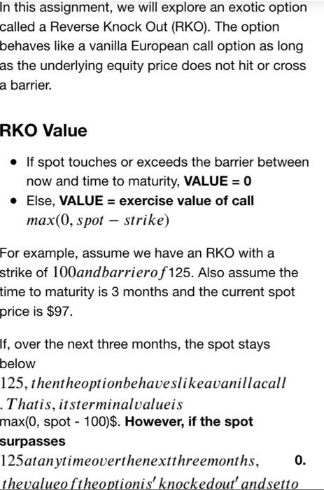
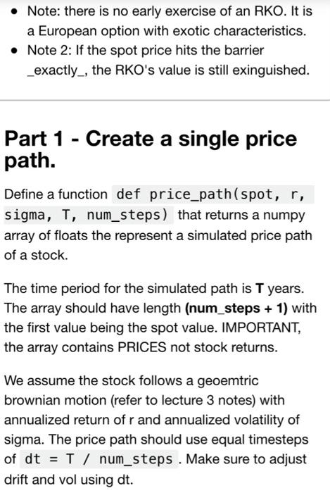
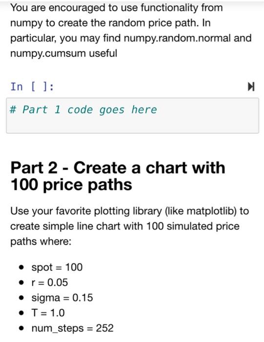
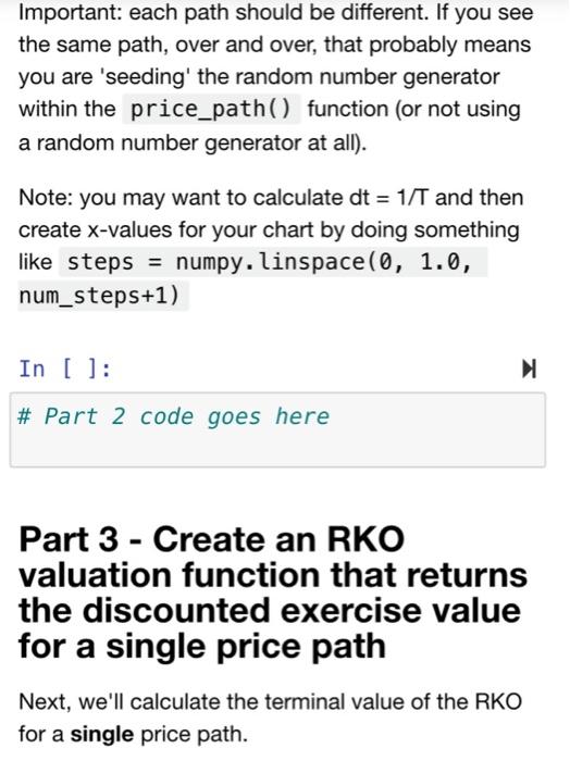
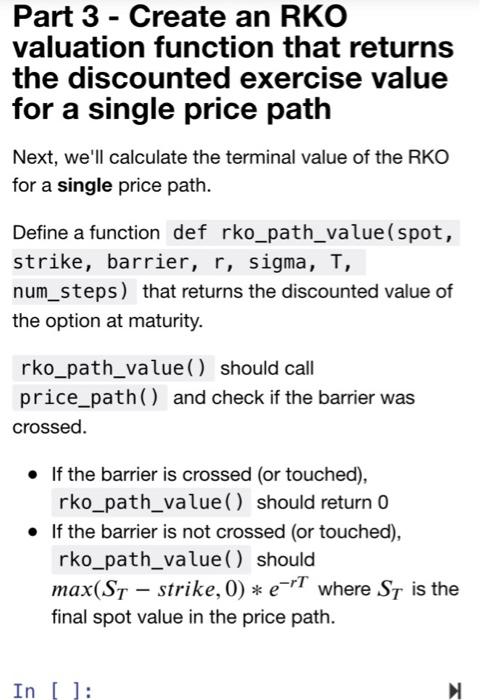
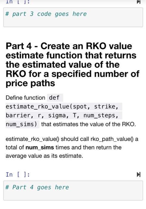
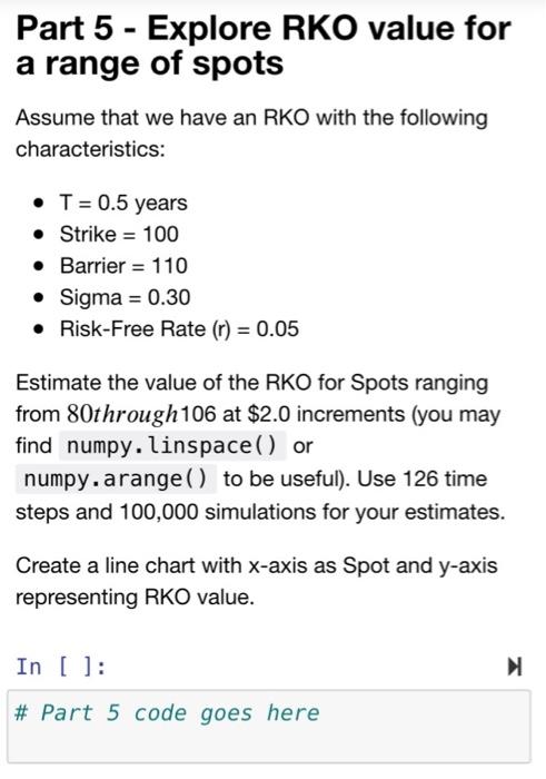
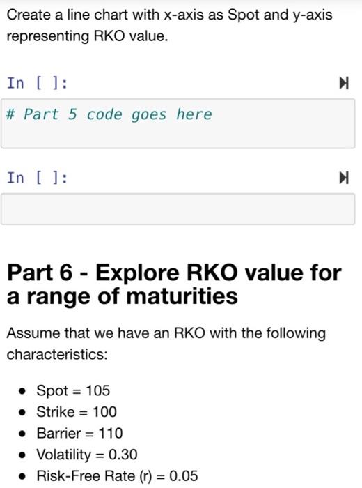
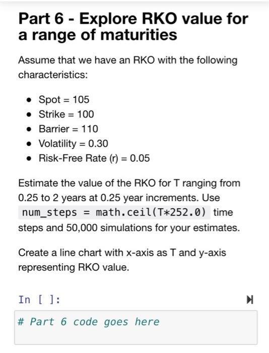
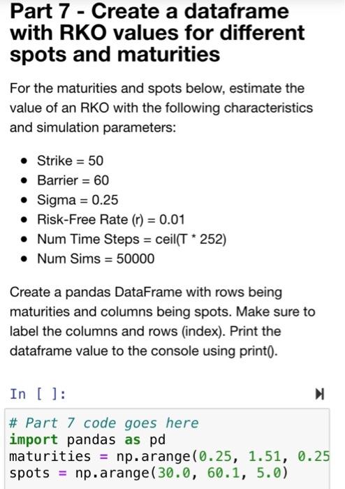
In this assignment, we will explore an exotic option called a Reverse Knock Out (RKO). The option behaves like a vanilla European call option as long as the underlying equity price does not hit or cross a barrier. RKO Value If spot touches or exceeds the barrier between now and time to maturity, VALUE = 0 Else, VALUE = exercise value of call max(0, spot - strike) For example, assume we have an RKO with a strike of 100andbarrierof 125. Also assume the time to maturity is 3 months and the current spot price is $97. If, over the next three months, the spot stays below 125, thentheoptionbehaveslikeavanillacall .Thatis, itsterminalvalueis max(0, spot - 100)$. However, if the spot surpasses 125atanytimeoverthenextthreemonths, 0. thevalueoftheoptionis' knockedout' and setto Note: there is no early exercise of an RKO. It is a European option with exotic characteristics. Note 2: If the spot price hits the barrier _exactly, the RKO's value is still exinguished. Part 1 - Create a single price path. Define a function def price_path(spot, r, sigma, T, num_steps) that returns a numpy array of floats the represent a simulated price path of a stock. The time period for the simulated path is T years. The array should have length (num_steps + 1) with the first value being the spot value. IMPORTANT, the array contains PRICES not stock returns. We assume the stock follows a geoemtric brownian motion (refer to lecture 3 notes) with annualized return of r and annualized volatility of sigma. The price path should use equal timesteps of dt = T / num_steps . Make sure to adjust drift and vol using dt. You are encouraged to use functionality from numpy to create the random price path. In particular, you may find numpy.random.normal and numpy.cumsum useful In [ ]: ] # Part 1 code goes here Part 2 - Create a chart with 100 price paths Use your favorite plotting library (like matplotlib) to create simple line chart with 100 simulated price paths where: spot = 100 r = 0.05 sigma = 0.15 T = 1.0 num_steps = 252 Important: each path should be different. If you see the same path, over and over, that probably means you are 'seeding' the random number generator within the price_path() function (or not using a random number generator at all). Note: you may want to calculate dt = 1/T and then create x-values for your chart by doing something like steps = numpy.linspace(0, 1.0, num_steps+1) In [ ]: # Part 2 code goes here Part 3 - Create an RKO valuation function that returns the discounted exercise value for a single price path Next, we'll calculate the terminal value of the RKO for a single price path. Part 3 - Create an RKO valuation function that returns the discounted exercise value for a single price path Next, we'll calculate the terminal value of the RKO for a single price path. Define a function def rko_path_value( spot, strike, barrier, r, sigma, T, num_steps) that returns the discounted value of the option at maturity. rko_path_value() should call price_path() and check if the barrier was crossed. If the barrier is crossed (or touched), rko_path_value() should return 0 If the barrier is not crossed (or touched), rko_path_value() should max(ST - strike, 0) * e-T where Sy is the final spot value in the price path. In [ ]: in LJ: 1 # part 3 code goes here Part 4 - Create an RKO value estimate function that returns the estimated value of the RKO for a specified number of price paths Define function def estimate_rko_value( spot, strike, barrier, r, sigma, T, num_steps, num_sims) that estimates the value of the RKO. estimate_rko_value() should call rko_path_value() a total of num_sims times and then return the average value as its estimate. In [ ]: # Part 4 goes here Part 5 - Explore RKO value for a range of spots Assume that we have an RKO with the following characteristics: T = 0.5 years Strike = 100 Barrier = 110 Sigma = 0.30 Risk-Free Rate (n) = 0.05 Estimate the value of the RKO for Spots ranging from 80through 106 at $2.0 increments (you may find numpy.linspace() or numpy.arange() to be useful). Use 126 time steps and 100,000 simulations for your estimates. Create a line chart with x-axis as Spot and y-axis representing RKO value. In [ ]: # Part 5 code goes here Create a line chart with x-axis as Spot and y-axis representing RKO value. In [ ]: # Part 5 code goes here In [ ]: N Part 6 - Explore RKO value for a range of maturities Assume that we have an RKO with the following characteristics: Spot = 105 Strike = 100 Barrier = 110 Volatility = 0.30 Risk-Free Rate (r) = 0.05 Part 6 - Explore RKO value for a range of maturities Assume that we have an RKO with the following characteristics: Spot = 105 Strike = 100 Barrier = 110 Volatility = 0.30 Risk-Free Rate (r) = 0.05 Estimate the value of the RKO for T ranging from 0.25 to 2 years at 0.25 year increments. Use num_steps = math.ceil(T*252.0) time steps and 50,000 simulations for your estimates. Create a line chart with x-axis as T and y-axis representing RKO value. In [ ]: # Part 6 code goes here Part 7 - Create a dataframe with RKO values for different spots and maturities For the maturities and spots below, estimate the value of an RKO with the following characteristics and simulation parameters: Strike = 50 Barrier = 60 Sigma = 0.25 Risk-Free Rate (n) = 0.01 Num Time Steps = ceil(T * 252) Num Sims = 50000 Create a pandas DataFrame with rows being maturities and columns being spots. Make sure to label the columns and rows (index). Print the dataframe value to the console using print(). In [ ]: # Part 7 code goes here import pandas as pd maturities = np.arange (0.25, 1.51, 0.25 spots = np.arange (30.0, 60.1, 5.0) In this assignment, we will explore an exotic option called a Reverse Knock Out (RKO). The option behaves like a vanilla European call option as long as the underlying equity price does not hit or cross a barrier. RKO Value If spot touches or exceeds the barrier between now and time to maturity, VALUE = 0 Else, VALUE = exercise value of call max(0, spot - strike) For example, assume we have an RKO with a strike of 100andbarrierof 125. Also assume the time to maturity is 3 months and the current spot price is $97. If, over the next three months, the spot stays below 125, thentheoptionbehaveslikeavanillacall .Thatis, itsterminalvalueis max(0, spot - 100)$. However, if the spot surpasses 125atanytimeoverthenextthreemonths, 0. thevalueoftheoptionis' knockedout' and setto Note: there is no early exercise of an RKO. It is a European option with exotic characteristics. Note 2: If the spot price hits the barrier _exactly, the RKO's value is still exinguished. Part 1 - Create a single price path. Define a function def price_path(spot, r, sigma, T, num_steps) that returns a numpy array of floats the represent a simulated price path of a stock. The time period for the simulated path is T years. The array should have length (num_steps + 1) with the first value being the spot value. IMPORTANT, the array contains PRICES not stock returns. We assume the stock follows a geoemtric brownian motion (refer to lecture 3 notes) with annualized return of r and annualized volatility of sigma. The price path should use equal timesteps of dt = T / num_steps . Make sure to adjust drift and vol using dt. You are encouraged to use functionality from numpy to create the random price path. In particular, you may find numpy.random.normal and numpy.cumsum useful In [ ]: ] # Part 1 code goes here Part 2 - Create a chart with 100 price paths Use your favorite plotting library (like matplotlib) to create simple line chart with 100 simulated price paths where: spot = 100 r = 0.05 sigma = 0.15 T = 1.0 num_steps = 252 Important: each path should be different. If you see the same path, over and over, that probably means you are 'seeding' the random number generator within the price_path() function (or not using a random number generator at all). Note: you may want to calculate dt = 1/T and then create x-values for your chart by doing something like steps = numpy.linspace(0, 1.0, num_steps+1) In [ ]: # Part 2 code goes here Part 3 - Create an RKO valuation function that returns the discounted exercise value for a single price path Next, we'll calculate the terminal value of the RKO for a single price path. Part 3 - Create an RKO valuation function that returns the discounted exercise value for a single price path Next, we'll calculate the terminal value of the RKO for a single price path. Define a function def rko_path_value( spot, strike, barrier, r, sigma, T, num_steps) that returns the discounted value of the option at maturity. rko_path_value() should call price_path() and check if the barrier was crossed. If the barrier is crossed (or touched), rko_path_value() should return 0 If the barrier is not crossed (or touched), rko_path_value() should max(ST - strike, 0) * e-T where Sy is the final spot value in the price path. In [ ]: in LJ: 1 # part 3 code goes here Part 4 - Create an RKO value estimate function that returns the estimated value of the RKO for a specified number of price paths Define function def estimate_rko_value( spot, strike, barrier, r, sigma, T, num_steps, num_sims) that estimates the value of the RKO. estimate_rko_value() should call rko_path_value() a total of num_sims times and then return the average value as its estimate. In [ ]: # Part 4 goes here Part 5 - Explore RKO value for a range of spots Assume that we have an RKO with the following characteristics: T = 0.5 years Strike = 100 Barrier = 110 Sigma = 0.30 Risk-Free Rate (n) = 0.05 Estimate the value of the RKO for Spots ranging from 80through 106 at $2.0 increments (you may find numpy.linspace() or numpy.arange() to be useful). Use 126 time steps and 100,000 simulations for your estimates. Create a line chart with x-axis as Spot and y-axis representing RKO value. In [ ]: # Part 5 code goes here Create a line chart with x-axis as Spot and y-axis representing RKO value. In [ ]: # Part 5 code goes here In [ ]: N Part 6 - Explore RKO value for a range of maturities Assume that we have an RKO with the following characteristics: Spot = 105 Strike = 100 Barrier = 110 Volatility = 0.30 Risk-Free Rate (r) = 0.05 Part 6 - Explore RKO value for a range of maturities Assume that we have an RKO with the following characteristics: Spot = 105 Strike = 100 Barrier = 110 Volatility = 0.30 Risk-Free Rate (r) = 0.05 Estimate the value of the RKO for T ranging from 0.25 to 2 years at 0.25 year increments. Use num_steps = math.ceil(T*252.0) time steps and 50,000 simulations for your estimates. Create a line chart with x-axis as T and y-axis representing RKO value. In [ ]: # Part 6 code goes here Part 7 - Create a dataframe with RKO values for different spots and maturities For the maturities and spots below, estimate the value of an RKO with the following characteristics and simulation parameters: Strike = 50 Barrier = 60 Sigma = 0.25 Risk-Free Rate (n) = 0.01 Num Time Steps = ceil(T * 252) Num Sims = 50000 Create a pandas DataFrame with rows being maturities and columns being spots. Make sure to label the columns and rows (index). Print the dataframe value to the console using print(). In [ ]: # Part 7 code goes here import pandas as pd maturities = np.arange (0.25, 1.51, 0.25 spots = np.arange (30.0, 60.1, 5.0) If its not clear from the pictures, Part 7, code box contains:
# Part 7 code goes here
import pandas as pd
maturities = np.arange(0.25, 1.51, 0.25)
spots = np.arange(30.0, 60.1, 5.0)


Step by Step Solution
There are 3 Steps involved in it
Step: 1

Get Instant Access to Expert-Tailored Solutions
See step-by-step solutions with expert insights and AI powered tools for academic success
Step: 2

Step: 3

Ace Your Homework with AI
Get the answers you need in no time with our AI-driven, step-by-step assistance
Get Started


