Question: PLEASE READ ALL THE LOCKED COMMENTS CAREFULLY BEFORE SUBMITTING ANY ANSWERS. N IF YOU DO NOT READ THESE COMMENTS, YOU ARE LIKELY TO OVERLOOK AN
![for Boyle's Law 11 Y = data_air( [6 11 16], [2:18]); %Selecting](https://s3.amazonaws.com/si.experts.images/answers/2024/06/667fd61f0765e_918667fd61ed9838.jpg)
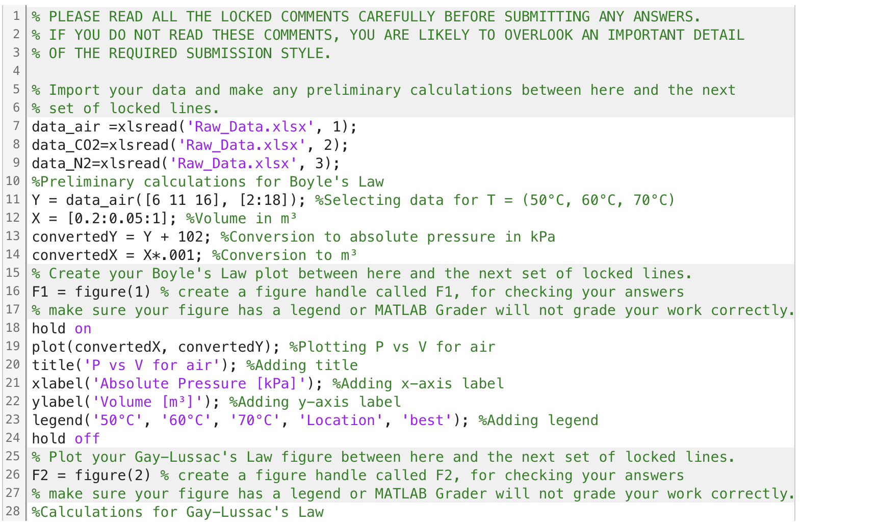
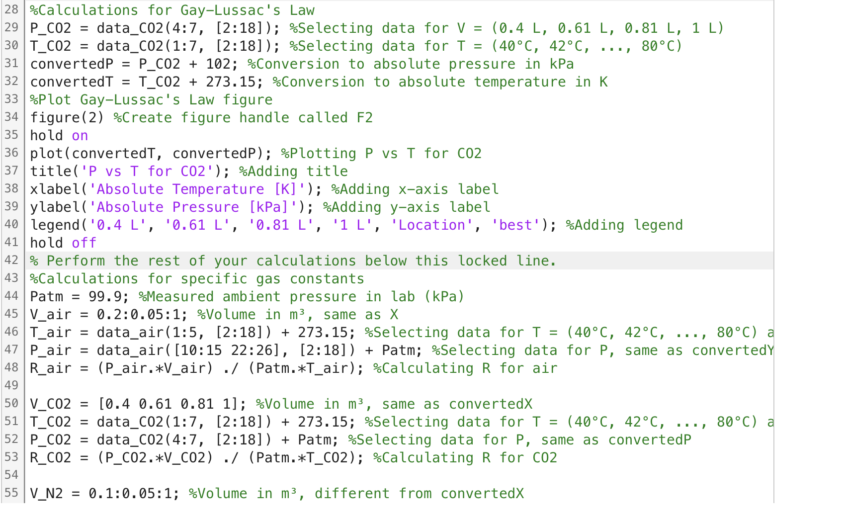
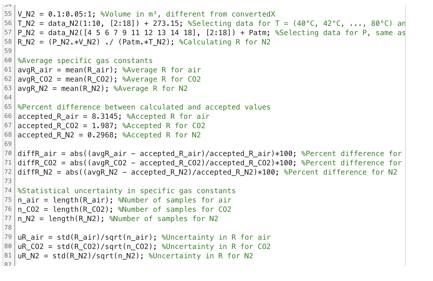
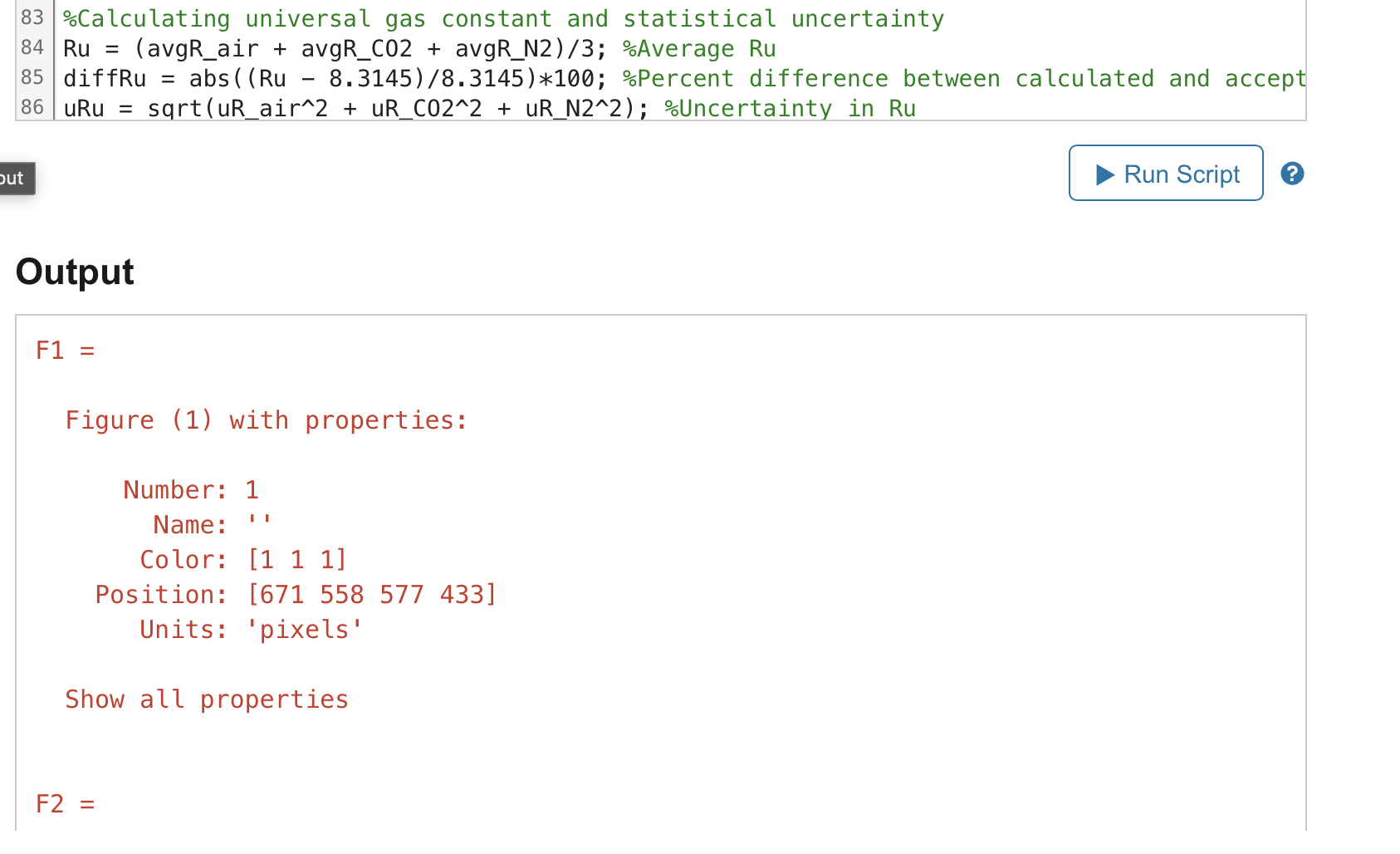
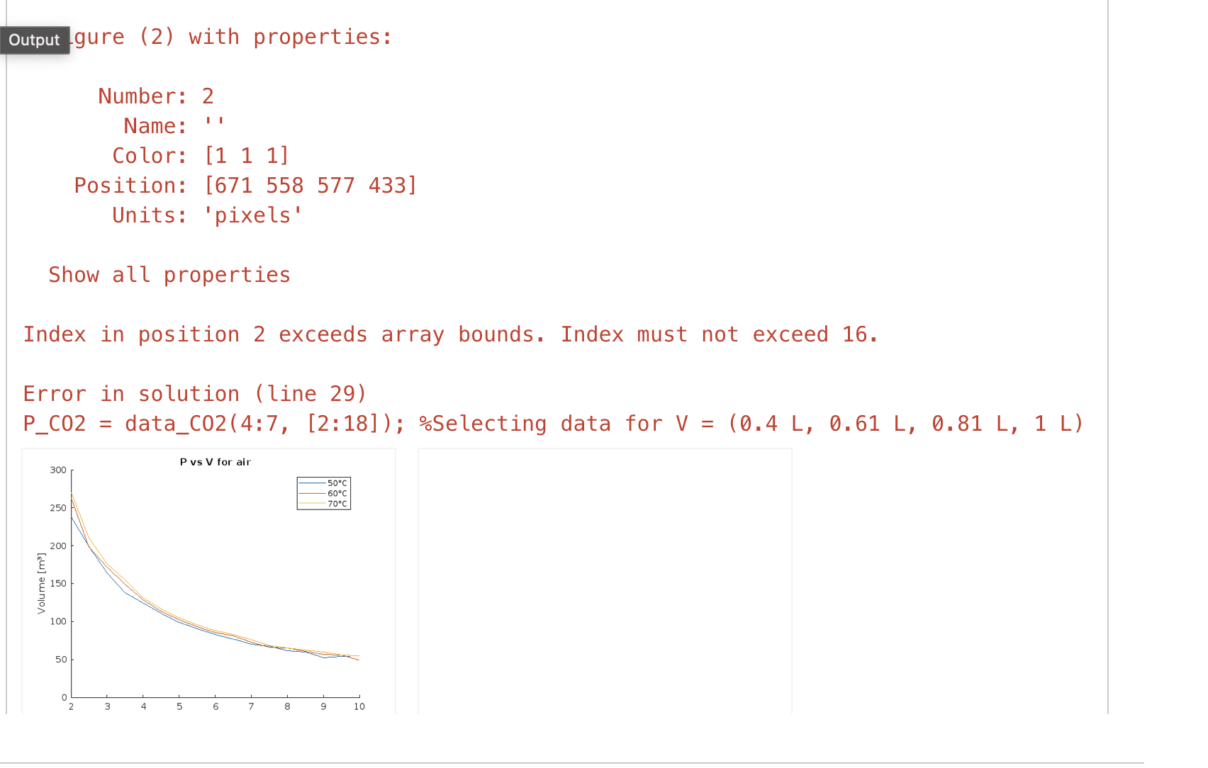
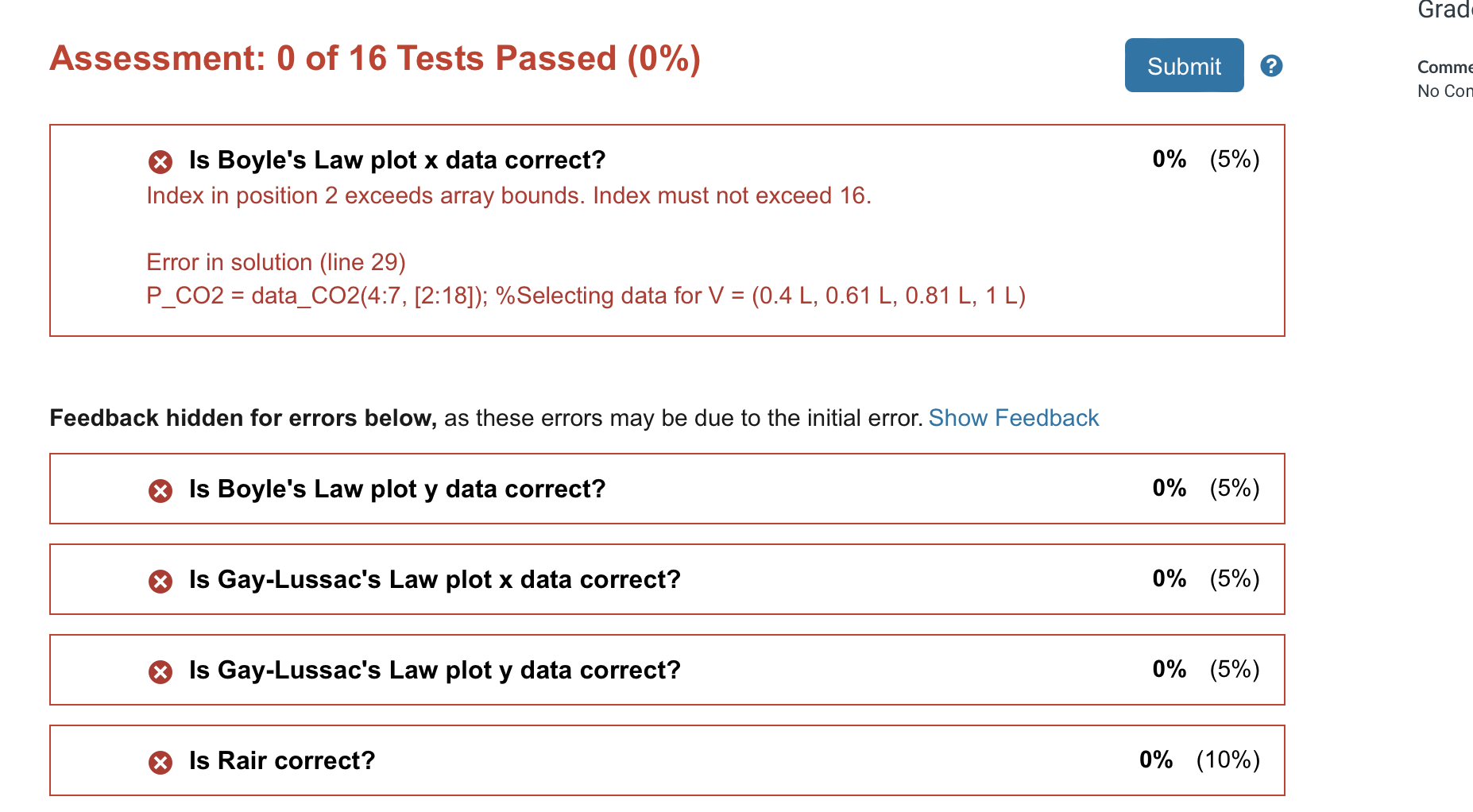
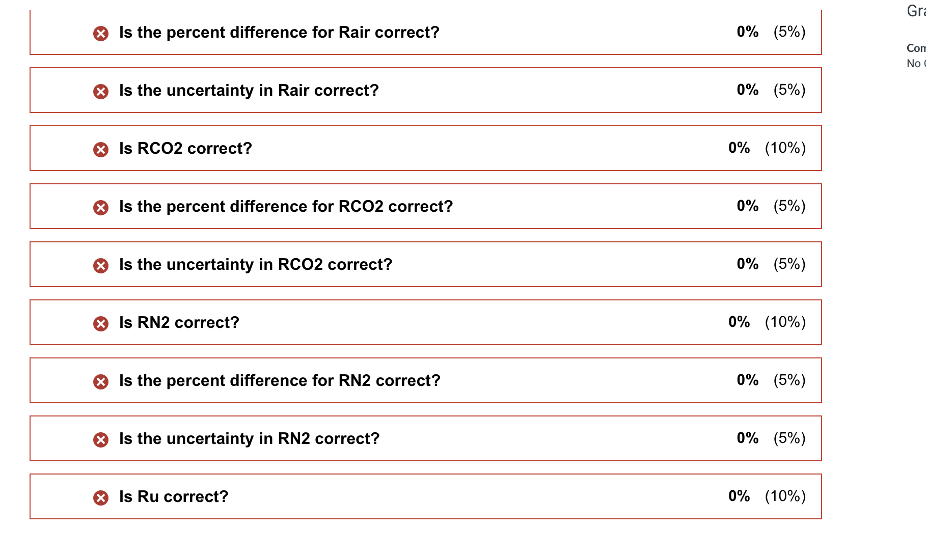
PLEASE READ ALL THE LOCKED COMMENTS CAREFULLY BEFORE SUBMITTING ANY ANSWERS. N IF YOU DO NOT READ THESE COMMENTS, YOU ARE LIKELY TO OVERLOOK AN IMPORTANT DETAIL W OF THE REQUIRED SUBMISSION STYLE. 4 5 % Import your data and make any preliminary calculations between here and the next 6 " set of locked lines. data_air =xlsread( ' Raw_Data. xlsx' , 1) ; 8 data_C02=xlsread( ' Raw_Data . xlsx' , 2) ; 9 data_N2=xlsread( ' Raw_Data. xlsx' , 3) ; 10 Preliminary calculations for Boyle's Law 11 Y = data_air( [6 11 16], [2:18]); %Selecting data for T = (50.C, 60.C, 70.C) 12 X = [0. 2:0. 05:1] ; Volume in m3 13 convertedY = Y + 102; %Conversion to absolute pressure in kPa 14 convertedX = X*. 001; %Conversion to m3 15 Create your Boyle's Law plot between here and the next set of locked lines. 16 F1 = figure(1) % create a figure handle called F1, for checking your answers 17 make sure your figure has a legend or MATLAB Grader will not grade your work correctly. 18 hold on 19 plot (convertedX, convertedY) ; Plotting P vs V for air 20 title('P vs V for air'); Adding title 21 xlabel( 'Absolute Pressure [kPa] ' ); Adding x-axis label 22 ylabel( 'Volume [m3] ' ) ; Adding y-axis label 23 legend ( '50.C', '60 C', '70.C', 'Location', 'best' ); Adding legend 24 hold off 25 % Plot your Gay-Lussac's Law figure between here and the next set of locked lines. 26 F2 = figure(2) % create a figure handle called F2, for checking your answers 27 % make sure your figure has a legend or MATLAB Grader will not grade your work correctly. 28 Calculations for Gay-Lussac's Law28 Calculations for Gay-Lussac's Law 29 P_C02 = data_C02(4:7, [2:18] ); Selecting data for V = (0.4 L, 0.61 L, 0.81 L, 1 L) 30 T_C02 = data_C02(1:7, [2:18] ); Selecting data for T = (40.C, 42.C, . .., 80.() 31 convertedP = P_C02 + 102; Conversion to absolute pressure in kPa 32 convertedT = T_C02 + 273.15; Conversion to absolute temperature in K 33 Plot Gay-Lussac's Law figure 34 figure(2) Create figure handle called F2 35 hold on 36 plot (convertedT, convertedP); Plotting P vs T for C02 37 title('P vs T for C02' ); Adding title 38 xlabel( ' Absolute Temperature [K] ' ) ; Adding x-axis label 39 ylabel( 'Absolute Pressure [kPa] ' ) ; %Adding y-axis label 40 legend ( '0.4 L', '0.61 L', '0.81 L', '1 L', 'Location', 'best' ); "Adding legend 41 hold off 42 Perform the rest of your calculations below this locked line. 43 Calculations for specific gas constants Patm = 99.9; Measured ambient pressure in lab (kPa) 45 V_air = 0.2:0. 05:1; Volume in m3, same as X 46 T_air = data_air (1:5, [2:18] ) + 273.15; Selecting data for T = (40.C, 42.C, . . ., 80.() a 47 P_air = data_air ( [10:15 22:26], [2:18] ) + Patm; %Selecting data for P, same as convertedY 48 Rair = (P_air.*V_air) ./ (Patm. *T_air); Calculating R for air 49 50 V_CO2 = [0.4 0.61 0.81 1]; Volume in m3, same as convertedX 51 T_CO2 = data_C02(1:7, [2:18] ) + 273.15; %Selecting data for T = (40.C, 42.C, . . ., 80.() a 52 P_CO2 = data_C02(4:7, [2:18] ) + Patm; Selecting data for P, same as convertedP 53 R C02 = (P_C02.*V_CO2) ./ (Patm.*T_C02); %Calculating R for C02 54 55 V_N2 = 0. 1:0. 05:1; Volume in m3, different from convertedX55 V N2 = 0. 1:0. 05:1; Volume in m3, different from convertedX 56 T_N2 = data_N2(1:10, [2:18] ) + 273.15; %Selecting data for T = (40.C, 42.C, . .., 80.C) an 57 P_N2 = data_N2( [4 5 6 7 9 11 12 13 14 18], [2:18] ) + Patm; Selecting data for P, same as 58 R_N2 = (P_N2. *V_N2) ./ (Patm. *T_N2) ; Calculating R for N2 59 60 Average specific gas constants 61 avgR_air = mean (R_air) ; Average R for air 62 avgR_CO2 = mean (R_C02) ; %Average R for C02 63 avgR_N2 = mean (R_N2) ; %Average R for N2 64 65 Percent difference between calculated and accepted values 66 accepted_R_air = 8.3145; %Accepted R for air 67 accepted_R_C02 = 1.987; %Accepted R for C02 68 accepted_R_N2 = 0. 2968; %Accepted R for N2 69 70 diffR_air = abs ( (avgR_air - accepted_R_air) /accepted_R_air)*100; Percent difference for 71 diffR_C02 = abs ( (avgR_C02 - accepted_R_C02) /accepted_R_C02)*100; Percent difference for 72 diffR_N2 = abs ( (avgR_N2 - accepted_R_N2) /accepted_R_N2) *100; Percent difference for N2 73 74 Statistical uncertainty in specific gas constants 75 n air = length (R_air) ; Number of samples for air 76 In_C02 = length (R_CO2) ; Number of samples for CO2 77 n_N2 = length (R_N2) ; Number of samples for N2 78 79 uR_air = std(R_air) /sqrt(n_air); Uncertainty in R for air 80 UR_CO2 = std (R_C02) /sqrt (n_C02); Uncertainty in R for C02 81 UR_N2 = std(R_N2) /sqrt(n_N2); Uncertainty in R for N2 8283 Calculating universal gas constant and statistical uncertainty 84 Ru = (avgR_air + avgR_C02 + avgR_N2) /3; %Average Ru 85 diffRu = abs ( (Ru - 8.3145) /8.3145)*100; Percent difference between calculated and accept 86 uRu = sqrt (uR_air 2 + UR_CO2^2 + UR_N2^2) ; Uncertainty in Ru but Run Script Output F1 = Figure (1) with properties: Number: 1 Name : Color: [1 1 1] Position: [671 558 577 433] Units: 'pixels' Show all properties F2 =Output gure (2) with properties: Number: 2 Name : I I Color: [1 1 1] Position: [671 558 577 433] Units: 'pixels' Show all properties Index in position 2 exceeds array bounds. Index must not exceed 16. Error in solution (line 29) P_CO2 = data_C02(4:7, [2:18] ); Selecting data for V = (0.4 L, 0.61 L, 0.81 L, 1 L) P vs V for air 300 50.C 60.C 250 70 C 200 Volume [m]] 150 100 50 5 6 7 8 9 10Grad Assessment: 0 of 16 Tests Passed (0%) Comme No Con Is Boyle's Law plot x data correct? 0% (5%) Index in position 2 exceeds array bounds. Index must not exceed 16. Error in solution (line 29) P_CO2 = data_C02(4:7, [2:18]); %Selecting data for V= (0.4 L,0.61L,0.81L,1L) Feedback hidden for errors below, as these errors may be due to the initial error. Show Feedback Is Boyle's Law plot y data correct? 0% (5%) @ Is Gay-Lussac's Law plot x data correct? 0% (5%) ' Is Gay-Lussac's Law plot y data correct? 0% (5%) Is Rair correct? 0% (10%) Gr X Is the percent difference for Rair correct? 0% (5%) Cor No X Is the uncertainty in Rair correct? 0% (5%) X Is RCO2 correct? 0% (10%) X Is the percent difference for RCO2 correct? 0% (5%) X Is the uncertainty in RCO2 correct? 0% (5%) X Is RN2 correct? 0% (10%) X Is the percent difference for RN2 correct? 0% (5%) X Is the uncertainty in RN2 correct? 0% (5%) X Is Ru correct? 0% (10%)Experimental Procedure Fixed masses of 3 different gases (mass values in Appendix A) have been isolated in 3 different containers (Figure 1). The containers are well sealed, preventing any leakage, and each container is fitted with a piston that can be locked in place, allowing you to fix the container volume. Lockable Piston Pressure Taj Temperature Taj p > P p Containing Cylinder Isolated Ideal Gas Figure 1. Experimental apparatus for studying ideal gases. A fixed mass of an ideal gas is isolated in a containing cylinder fitted with a lockable piston, providing a means for altering the volume of the ideal gas. The cylinder is also fitted with temperature and pressure taps to measure these properties, as well. Perform the following steps to collect your data. 1. Select the container labeled \"Air\". 2. Unlock the piston stop and set the container volume to 0.2 L. Lock the piston in place. 3. Place the container on top of a hot plate. 4. Connect a thermocouple reader to the thermocouple wire protruding from the side of the container. Also connect the pressure-sensing tube to a diaphragm-type pressure gauge. 5. Set the hot plate to 40C. Wait ~3 minutes for the gas temperature to stabilize. The gas temperature will likely stabilize in the range of 36 - 38C, depending on the temperature in the lab on the day you are running your experiment. 6. Increase the set temperature on the hot plate by the difference between the target temperature and the stable gas temperature. Wait for the temperature to stabilize then repeat step 6 if necessary. 8. Record the pressure at the fixed volume and temperature. Note that the pressure gauge measures the gauge pressure of the gas: Pyauge = Pabsolute Patm, in kPa, where the subscript 'atm' represents the ambient pressure. 9. Repeat steps 5 -8 for {T | T [40C, 80C]} in increments of 2C. 10. Repeat steps 2 -9 for {V | V [0.2 L,1 L]} in increments of 0.05 L. 1. Repeat this experiment for CO, and N, with the following adjustments: a. For CO,, use{V |V [0.3 L,1L]} and the same temperature range. b. ForN,, use {V |V [0.1L,1L]}and the same temperature range. Analysis Use the raw data provided in the Excel file \"Raw_Data.xIxs\" to perform the analyses outlined below. This data file contains pressure measurements at each pair of temperature and volume values, P(V,T), described in the Experimental Procedure section above. 1. Visually verify Boyle's Law by plotting P vs V for air, where P is the absolute pressure in kPa and V is in m'. Your plot should contain 3 different lines representing T = {50C, 60C, 70C}. 2. Visually verify Gay-Lussac's Law by plotting P vs T for CO., where P is the absolute pressure in kPa and T in in C. Your plot should contain 4 different lines representing V = {0.4 L, 06L, 0.8L, 1L}. 3. Use the measured pressure data to calculate the average value of the specific gas constant (R) m?3 for each gas, in units of [%]A Don't forget that you must use absolute temperature and pressure in the Ideal Gas Law. The measured ambient pressure in the lab while you performed you experiments can be found in Appendix A. Call these variables Rair, RCO2, and RNz, respectively. 4. Calculate the percent difference between your calculated values of R and the accepted values (Appendix B). Call these variables diffRair, diffRCO2, and diffRN2. Use the percent difference as defined by accepted value calculated value % diff = b accepted value *100 5. Calculate the statistical uncertainty in the specific gas constant for each gas. Call these variables uRair, uRCO2, and uRNz, respectively. See Appendix C for a short discussion on making this calculation. 6. Repeat the average, percent difference, and statistical uncertainty calculations for the universal gas constant, in units of [kml;]'_K], using the data across all 3 gases. Call these variables Ru, diffRu, and uRu. Note: You will have to account for the fact that there are a different number of samples (data points) for each of the gases in your analysis. To see why this matters, consider the two arrays x; and x;: x =[3333333333333], x,=[2] The mean of each of these arrays is ] = 3 and X; = 2, respectively. We might naively presume that we can calculate the mean value of the entire set of data, x; U x,, where U represents the \"union\" of the two sets, as AT xnUx, = '2 2 =25 'We can clearly see that this is wrong, however, since X; U x; should be much closer to 3 than to 2. You must think carefully about how to properly incorporate all the data when performing these universal gas constant calculations
Step by Step Solution
There are 3 Steps involved in it

Get step-by-step solutions from verified subject matter experts


