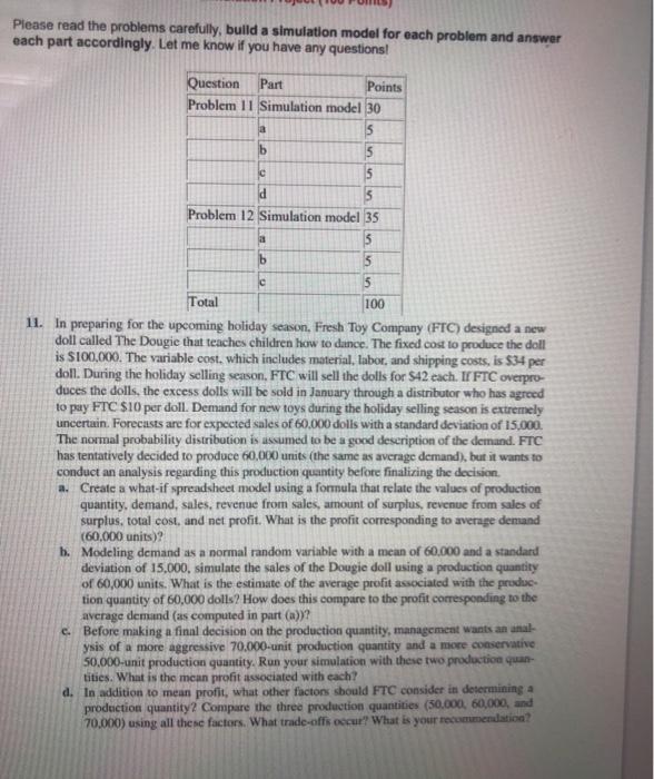
Please read the problems carefully, build a simulation model for each problem and answer each part accordingly. Let me know if you have any questions! Question Points Problem 1 1 Simulation model 30 15 Problem 12 Simulation model 35 Total 100 11. In preparing for the upcoming holiday season. Fresh Toy Company (FTC) designed a new doll called The Dougie that teaches children how to dance. The fixed cost to produce the doll is $100,000. The variable cost. which includes material, labor, and shipping costs, is $34 per doll. During the holiday selling season, FTC will sell the dolls for $42 each. II FTC overpro- duces the dolls, the excess dolls will be sold in January through a distributor who has agreed to pay FTC $10 per doll. Demand for new toys during the holiday selling season is extremely uncertain. Forecasts are for expected sales of 60,000 dolls with a standard deviation of 15,000 The normal probability distribution is assumed to be a good description of the demand. FTC has tentatively decided to produce 60,000 units (the same as average demand), but it wants to conduct an analysis regarding this production quantity before finalizing the decision. a. Create a what-if spreadsheet model using a formula that relate the values of production quantity. demand, sales, revenue from sales, amount of surplus, revenue from sales of surplus. total cost, and net profit. What is the profit corresponding to average demand (60,000 units)? Modeling demand as a normal random variable with a mean of 60.000 and a standard deviation of 15,000, simulate the sales of the Dougie doll using a production quantity of 60,000 units. What is the estimate of the average profit associated with the produc- tion quantity of 60,000 dolls? How does this compare to the profit corresponding to the average demand (as computed in part (a))? C. Before making a final decision on the production quantity, management wants an anal- ysis of a more aggressive 70.000-unit production quantity and a more conservative 50.000-unit production quantity. Run your simulation with these two production quan- tities. What is the mean profit associated with each? d. In addition to mean profit, what other factors should FTC consider in determining a production quantity? Compare the three production quantities (30,000, 60,000, and 70,000) using all these factors. What trade-offs occur? What is your recommendation?Example 5.6 A company is considering drilling four oil wells. The probability of success for each well is 0.40, independent of the results for any other well. The cost of each well is $200,000. Each well that is successful will be worth $600,000. a) What is the probability that one or more wells will be successful? b) What is the expected number of successes? c) What is the expected gain? d) What will be the gain if only one well is successful? e) Considering all possible results. what is the probability of a loss rather than a gain? What is the standard deviation of the number of successes?Example 13.5 Results of a study of the repair records of three models of cars over the first three years of the cars' lives on the basis of a sample are shown below. Percentages Requiring Car Model Number Surveyed Major Repairs Minor Repairs No Repairs A 20 50 30 B 30 40 40 20 C 40 30 60 10 333Example 9.10 We decide to run a test using an experimental evaporation pan and a standard evaporation pan over ten successive days. The two types are set up side-by-side so 238 Statistical Inferences for the Mean that atmospheric conditions should be the same. A coin is tossed to decide which evaporation pan is on the lefthand side and which on the righthand side on any particular day. The measured daily evaporations are as follows: Pair or Day No. 1 2 3 4 5 6 7 8 9 10 Evaporation, mm: Pan A 9.1 4.6 14.0 16.9 11.4 10.7 27.4 22.8 42.8 29.4 Pan B 6.7 3.1 13.8 16.6 12.3 6.5 24.2 20.1 41.9 27.7 d = Agym. A - B 2.4 1.5 0.2 0.3 -0.9 4.2 3.2 2.7 0.9 1.7 Does the experimental Pan A give significantly higher evaporation than the standard Pan B at the 1% level of significance?Example 9.7 The electrical resistances of components are measured as they are produced. A sample of six items gives a sample mean of 2.62 ohms and a sample standard devia- tion of 0.121 ohms. At what observed level of significance is this sample mean significantly different from a population mean of 2.80 ohms? Is there less than 2% probability of getting a sample mean this far away from 2.80 ohms or farther purely by chance when the population mean is 2.80 ohms?Example 10.3 Two additives to Portland cement are being tested for their effect on the strength of concrete. 21 batches were made with Additive A, and their strengths showed standard deviation s, = 41.3. 16 batches were made with the same percentage of Additive B. and their strengths showed standard deviation s, = 26.2. Assume that the strengths of concrete follow a normal distribution. Is there evidence at the 1% level of signifi- cance that the concrete made with Additive A is more variable than concrete made with Additive B?Example 12.3 Concrete specimens are made using three different experimental additives. The purpose of the additives is to try to accelerate the gain of strength as the concrete sets. All specimens have the same mass ratio of additive to Portland cement, and the same mass ratio of aggregate to cement, but three different mass ratios of water to cement. Two replicate specimens are made for each of nine combinations of factors, All specimens are kept under standard conditions. After twenty-eight days the compression strengths of the specimens are measured. The results (in MPa) are shown in Table 12.9. Table 12.9: Strengths of Concrete Specimens Additives Ratio, water #1 #2 #3 to cement Compressive Strengths 0.45 40.7 42.5 40.4 39 9 41.4 41.7 0.55 36 35.6 26.6 26.3 30.7 28.2 0.65 24.7 30.6 21.9 23.9 23.9 27.6 Do these data provide evidence that the additives or the water:cement ratios or interactions of the two affect the yield strength? Use the 5% level of significance
