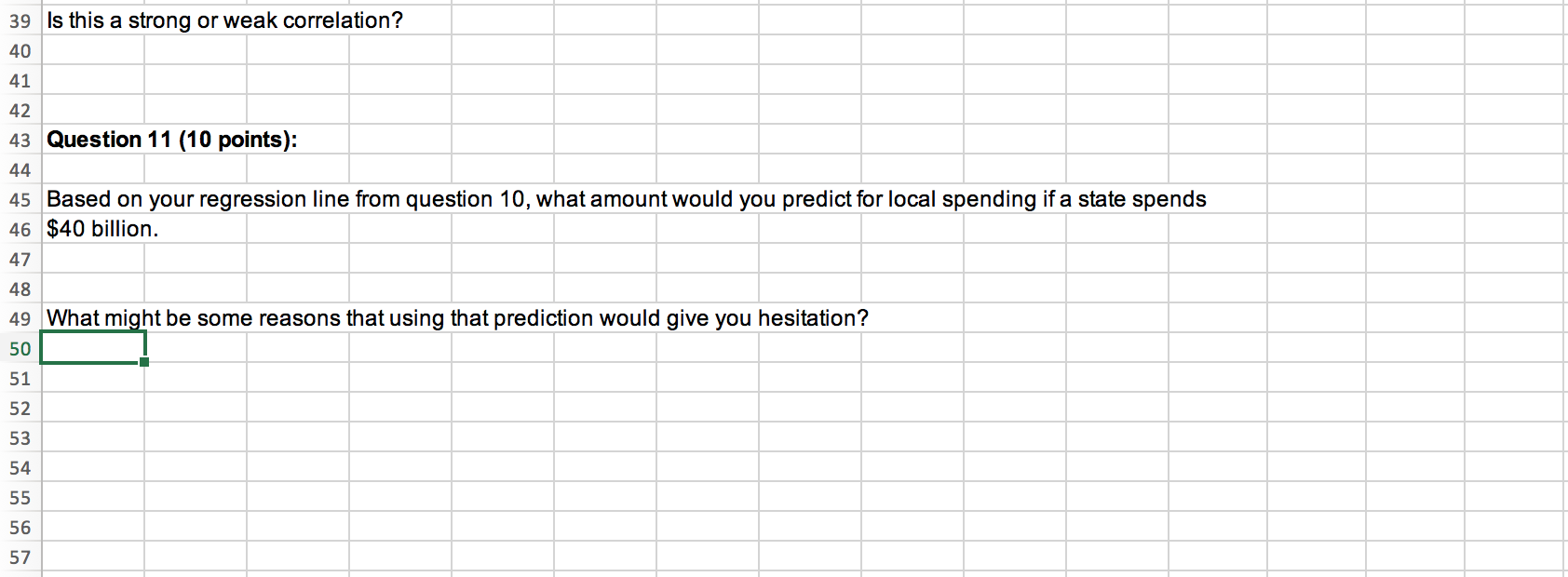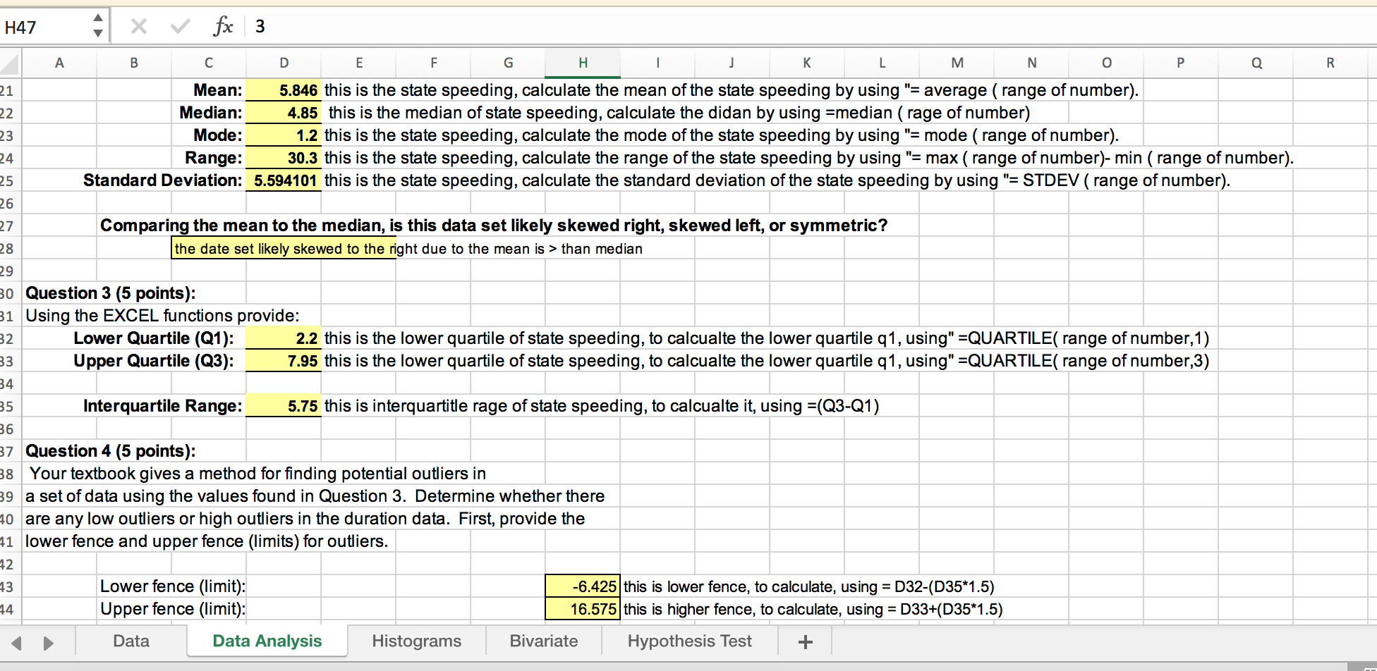


Please scroll from to bottom to the top
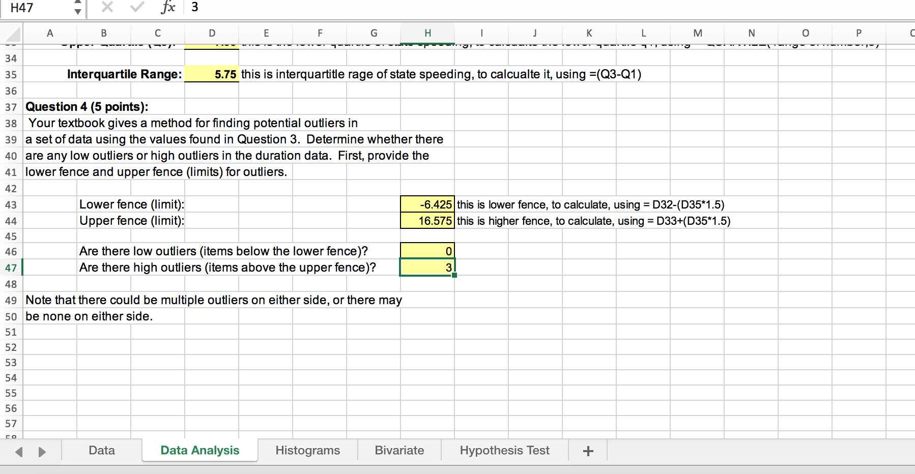
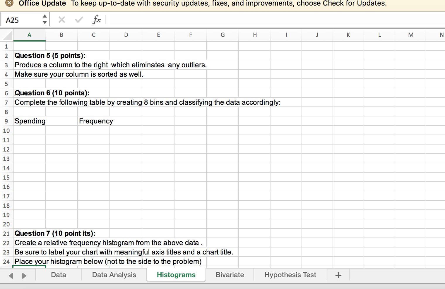
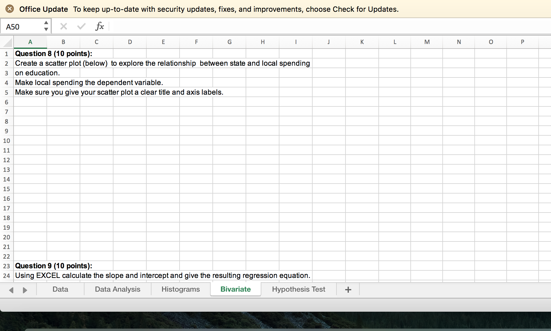
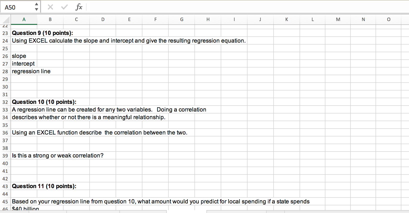
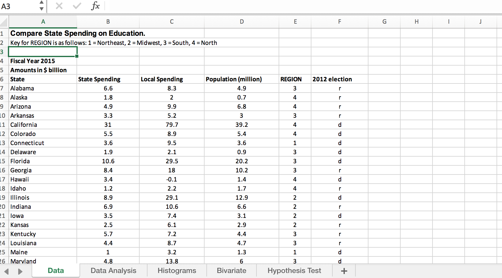
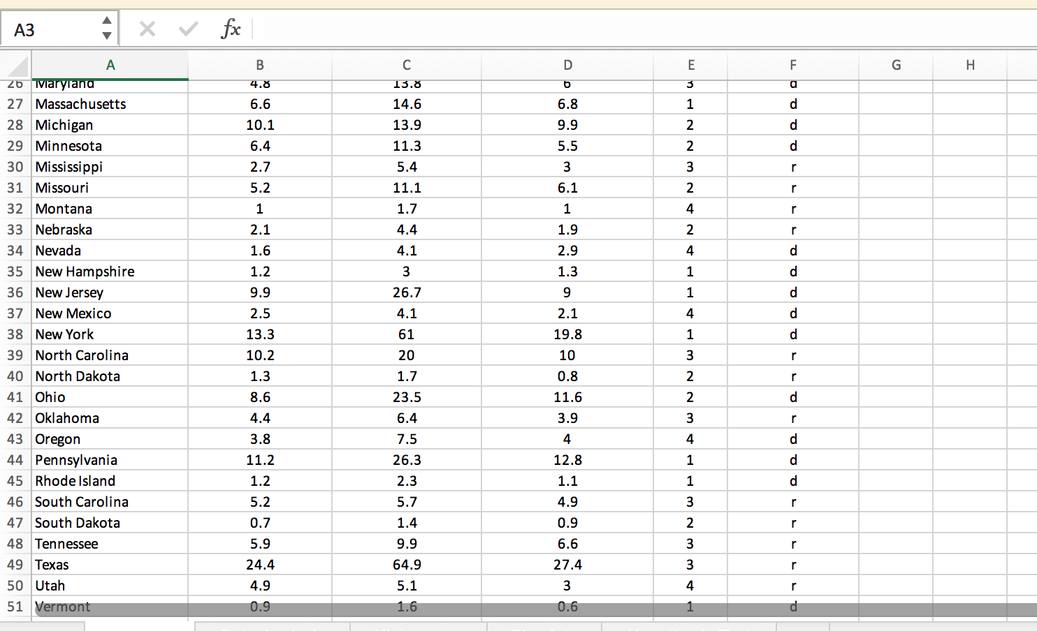
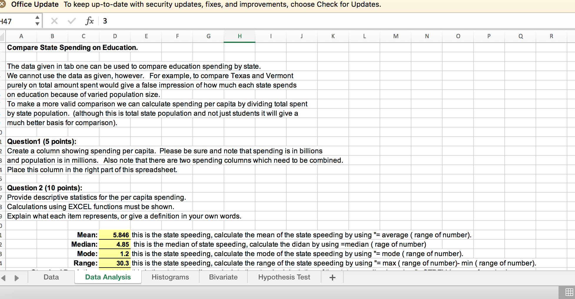
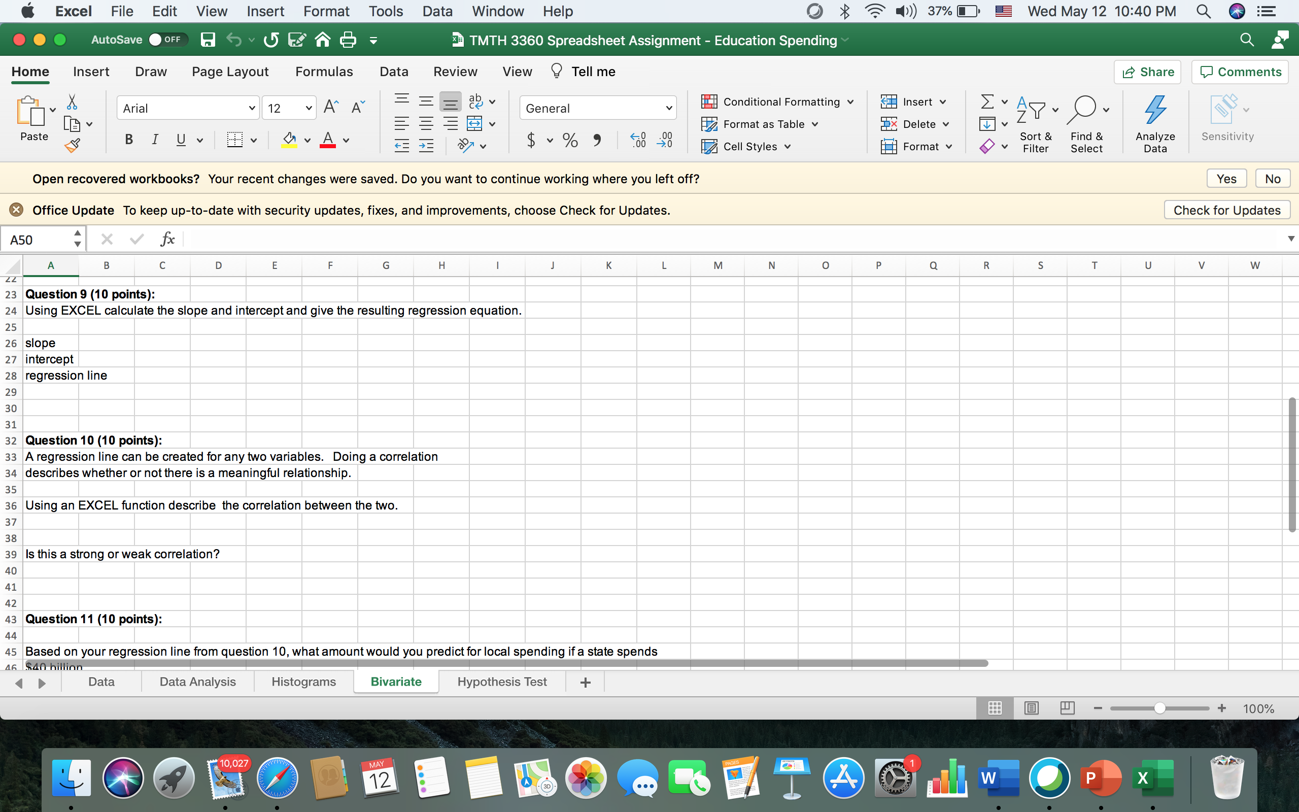
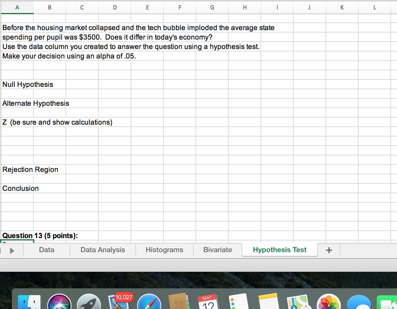
A3 X V fx A B C D E F G H Compare State Spending on Education. Key for REGION is as follows: 1 = Northeast, 2 = Midwest, 3 = South, 4 = North Fiscal Year 2015 Amounts in $ billion State State Spending Local Spending Population (million) REGION 2012 election Alabama 6.6 8.3 4.9 3 r Alaska 1.8 2 0.7 Arizona 4.9 9.9 6.8 W A 0 Arkansas 3.3 5.2 3 1 California 31 79.7 39.2 .2 Colorado 5.5 8.9 5.4 3 Connecticut 3.6 9.5 3.6 Delaware 1.9 2.1 0.9 5 Florida 10.6 29.5 20.2 6 Georgia 8.4 18 10.2 7 Hawaii 3.4 -0.1 1.4 8 Idaho 1.2 2.2 1.7 9 Illinois 8.9 29.1 12.9 0 Indiana 6.9 10.6 6.6 lowa 3.5 7.4 3.1 Kansas 2.5 6.1 2.9 W H WWNNNN. 3 Kentucky 5.7 7.2 4.4 4 Louisiana 4.4 8.7 4.7 5 Maine 1 3.2 1.3 6 Marvland 4.8 13.8 6 Data Data Analysis Histograms Bivariate Hypothesis Test +A3 X V fx A B C D G H 26 Maryland 4.8 13.8 27 Massachusetts 6.6 14.6 6.8 28 Michigan 10.1 13.9 9.9 29 Minnesota 6.4 11.3 5.5 30 Mississippi 2.7 ANANWNNHUM 5.4 3 31 Missouri 5.2 11.1 6.1 32 Montana 1 1.7 1 33 Nebraska 2.1 4.4 1.9 34 Nevada 1.6 4.1 2.9 35 New Hampshire 1.2 3 1.3 36 New Jersey 9.9 26.7 9 37 New Mexico 2.5 4.1 2.1 38 New York 13.3 61 19.8 39 North Carolina 10.2 20 10 AWNNW HAPPY 40 North Dakota 1.3 1.7 0.8 41 Ohio 8.6 23.5 11.6 42 Oklahoma 4.4 6.4 3.9 Oregon 3.8 7.5 4 44 Pennsylvania 11.2 26.3 12.8 45 Rhode Island 1.2 2.3 1.1 46 South Carolina 5.2 5.7 4.9 47 South Dakota 0.7 1.4 0.9 A W W N WHY Tennessee 5.9 9.9 6.6 Texas 24.4 64.9 27.4 50 Utah 4.9 5.1 3 51 Vermont 0.9 1.6 0.6Office Update To keep up-to-date with security updates, fixes, and improvements, choose Check for Updates. 147 X V fx 3 A B C D E F G H K L M N O P Q R Compare State Spending on Education. The data given in tab one can be used to compare education spending by state. We cannot use the data as given, however. For example, to compare Texas and Vermont purely on total amount spent would give a false impression of how much each state spends on education because of varied population size. To make a more valid comparison we can calculate spending per capita by dividing total spent by state population. (although this is total state population and not just students it will give a much better basis for comparison). Question1 (5 points): Create a column showing spending per capita. Please be sure and note that spending is in billions and population is in millions. Also note that there are two spending columns which need to be combined. Place this column in the right part of this spreadsheet. Question 2 (10 points): Provide descriptive statistics for the per capita spending. Calculations using EXCEL functions must be shown. Explain what each item represents, or give a definition in your own words. Mean: 5.846 this is the state speeding, calculate the mean of the state speeding by using "= average ( range of number). Median: 4.85 this is the median of state speeding, calculate the didan by using =median ( rage of number) Mode: 1.2 this is the state speeding, calculate the mode of the state speeding by using "= mode ( range of number). Range: 30.3 this is the state speeding, calculate the range of the state speeding by using "= max ( range of number)- min ( range of number). Data Data Analysis Histograms Bivariate Hypothesis Test +H47 X V fx 3 A B C D E F G H K M N O P Q R 21 Mean: 5.846 this is the state speeding, calculate the mean of the state speeding by using "= average ( range of number). 2 Median: 4.85 this is the median of state speeding, calculate the didan by using =median ( rage of number) 3 Mode: 1.2 this is the state speeding, calculate the mode of the state speeding by using "= mode ( range of number). Range: 30.3 this is the state speeding, calculate the range of the state speeding by using "= max ( range of number)- min ( range of number). Standard Deviation: 5.594101 this is the state speeding, calculate the standard deviation of the state speeding by using "= STDEV ( range of number). Comparing the mean to the median, is this data set likely skewed right, skewed left, or symmetric? 8 the date set likely skewed to the right due to the mean is > than median Question 3 (5 points): Using the EXCEL functions provide: 32 Lower Quartile (Q1): 2.2 this is the lower quartile of state speeding, to calcualte the lower quartile q1, using" =QUARTILE( range of number, 1) Upper Quartile (Q3): 7.95 this is the lower quartile of state speeding, to calcualte the lower quartile q1, using" =QUARTILE( range of number,3) Interquartile Range: 5.75 this is interquartitle rage of state speeding, to calcualte it, using =(Q3-Q1) 7 Question 4 (5 points): Your textbook gives a method for finding potential outliers in 9 a set of data using the values found in Question 3. Determine whether there 10 are any low outliers or high outliers in the duration data. First, provide the 1 lower fence and upper fence (limits) for outliers. .2 13 Lower fence (limit): -6.425 this is lower fence, to calculate, using = D32-(D35*1.5) 14 Upper fence (limit): 16.575 this is higher fence, to calculate, using = D33+(D35*1.5) Data Data Analysis Histograms Bivariate Hypothesis Test +H47 X V fx A B C D E F G H K M N O P 34 35 Interquartile Range: 5.75 this is interquartitle rage of state speeding, to calcualte it, using =(Q3-Q1) 36 37 Question 4 (5 points): 38 Your textbook gives a method for finding potential outliers in 39 a set of data using the values found in Question 3. Determine whether there 40 are any low outliers or high outliers in the duration data. First, provide the 41 lower fence and upper fence (limits) for outliers. 42 43 Lower fence (limit): -6.425 this is lower fence, to calculate, using = D32-(D35*1.5) 44 Upper fence (limit): 16.575 this is higher fence, to calculate, using = D33+(D35*1.5) 45 46 Are there low outliers (items below the lower fence)? 0 47 Are there high outliers (items above the upper fence)? 3 49 Note that there could be multiple outliers on either side, or there may 50 be none on either side. 51 52 53 54 55 56 57 co Data Data Analysis Histograms Bivariate Hypothesis Test +X Office Update To keep up-to-date with security updates, fixes, and improvements, choose Check for Updates. A25 X V fx A B C D E F G H K L M Question 5 (5 points): Produce a column to the right which eliminates any outliers. Make sure your column is sorted as well. UI 6 Question 6 (10 points): Complete the following table by creating 8 bins and classifying the data accordingly: 9 Spending Frequency 10 11 12 13 14 15 16 17 18 19 20 21 Question 7 (10 point its): 22 Create a relative frequency histogram from the above data . 23 Be sure to label your chart with meaningful axis titles and a chart title. 24 Place your histogram below (not to the side to the problem) Data Data Analysis Histograms Bivariate Hypothesis Test +6 Office Update To keep uptodate with security updates, fixes, and improvements, choose Check for Updates. A50 3 f3: A B c D E F G H I J K L M N o P Question 8 (10 points): Create a scatter plot (below) to explore the relationship between state and local spending on education. Make local spending the dependent variable. Make sure you give your scatter plot a clear title and axis labels. mmummthiI NMNNHHHHHHHHHDl mmuommummthrno Question 9 (10 points): Using EXCEL calculate the slope and intercept and give the resulting regression equation. N J; 4 p Data Data Analysis Histograms Bivariate Hypothesis Test + .))) It) 37% E. 5 Wed May12 10:40 PM .' Excel File Edit View Insert Format Tools Data Window Help 0 >3 TMTH 3360 Spreadsheet Assignment - Education Spendi Home Insert Draw Page Layout Formulas Data Review View 9 Tell me l8 Share " A V E = ~ ab .. i (_ flj v A v' 12 V' A A _ _ cg v General v E Conditional Formatting v [a Insert v Z v 9? v p v ; I: V I I : H V 3; Format as Table v E Delete v .1. v Paste _ o <.u j10 __ sort find analyze sensitivity _ v a cellstyles mg format filter select data open recovered workbooks your recent changes were saved. do you want to continue working where left off office update keep up-to-date with security updates fixes and improvements choose check for updates. l fx . s c d e f g h i j k m n o p q r t u w question points using excel calculate the slope intercept give resulting regression equation. line can be created any two variables. doing correlation describes whether or not there is meaningful relationship. an excequnction describe between this strong weak based on from what amount would predict local spending ifa state spends analysis histograms bivariate hypothesis test el il0 iiicd a50 x b interceptand ____ minke ___ _- function two. hat amountwould if _____ slate mi ht some reasons that prediction hesitation before housing market collapsed tech bubble imploded average per pupil was does it differ in today economy use column answer test. make decision alpha of .05. null alternate sure show calculations rejection region conclusion>

