Please see attachment. thank you. work out only a part will be fine too

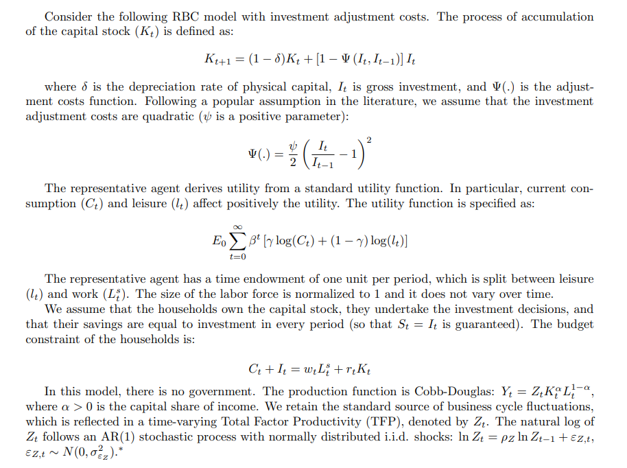
3. Now consider the steady-state of the model in the following four cases, where we change some parameter values (While keeping all the others at the benchmark calibration of point 2). Report, comment and interpret your results, stressing the economic mechanisms at play. (a) 3 = 0.98 (b) 7 = 0-3 (c) 6 = 0.03 ) (d 1J1 = 5.0 Consider the following RBC model with investment adjustment costs. The process of accumulation of the capital stock (K) is defined as: Kt+1 = (1 - 8) K+ + [1 - V (It, It-1) ] It where o is the depreciation rate of physical capital, It is gross investment, and V(.) is the adjust- ment costs function. Following a popular assumption in the literature, we assume that the investment adjustment costs are quadratic (? is a positive parameter): " ( . ) = It NIE The representative agent derives utility from a standard utility function. In particular, current con- sumption (Ct) and leisure (4) affect positively the utility. The utility function is specified as: Eo Bt [y log(Ct) + (1 - y) log(4t)] 1=0 The representative agent has a time endowment of one unit per period, which is split between leisure (It) and work (Lf). The size of the labor force is normalized to 1 and it does not vary over time. We assume that the households own the capital stock, they undertake the investment decisions, and that their savings are equal to investment in every period (so that St = It is guaranteed). The budget constraint of the households is: Ct the = weLitreKt In this model, there is no government. The production function is Cobb-Douglas: Yt = Z+KAL, -, where a > 0 is the capital share of income. We retain the standard source of business cycle fluctuations, which is reflected in a time-varying Total Factor Productivity (TFP), denoted by Z. The natural log of Zt follows an AR(1) stochastic process with normally distributed i.i.d. shocks: In Zt = pz In Zt-1 + Ez,t, EZ,t ~ N(0, OFZ).*