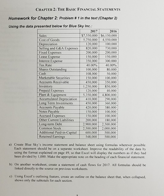
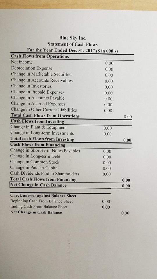
please show all work in Excel

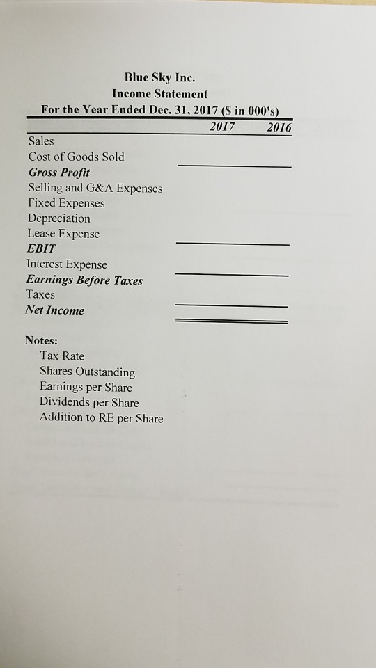
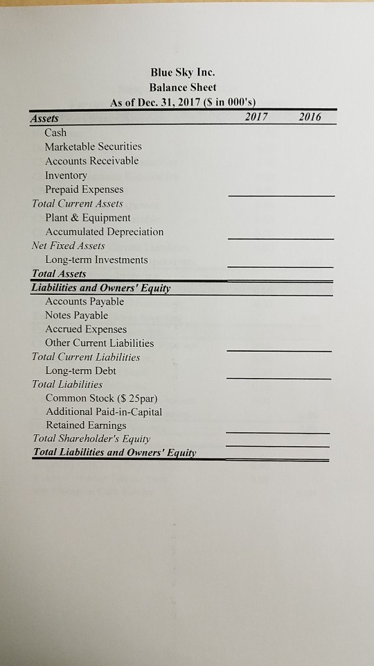
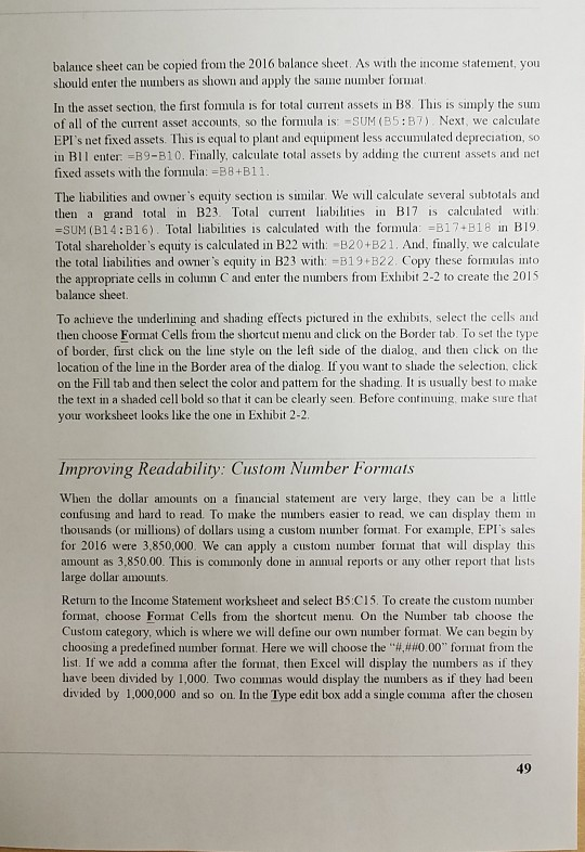
CHAPTER 2: THE BASIC FINANCIAL STATEMENTS Homework for Chapter 2: Problem # 1 in the text (Chapter 2) Using the data presented below for Blue Sky Inc.: 2017 2016 S7,550,000 $6,150,000 5,750,000 Sales Cost of Goods Depreciation Selling and G&A Expenses Fixed Expenses Lease Expense Interest Expense 4,550,000 120,000 100,000 820,000 730,000 200,000 200,000 150,000 150,000 350,000 300,000 Tax Rate 40.00% 40.00% Shares Outstanding Cash Marketable Securities Accounts Receivable Inventory Prepaid Expenses Plant & Equipment Accumulated Depreciation Long Term Investments Accounts Payable Notes Payable Accrued Expenses Other Current Liabilities Long-term Debt Common Stock Additional Paid-in-Capital Retained Earnings 100,000 108,000 80,000 50,000 150,000 100,000 450,000 350,000 1,250,000 850,000 40,000 120,000 5,350.000 4,800,000 290,000 410,000 450,000 360,000 420,000 380.000 150,000 150,000 200.000 100,000 100,000 180,000 2.900,000 2,500,000 2,500,000 2,000,000 600,000 500,000 548,000 500,000 a) Create Blue Sky's income statement and balance sheet using formulas wherever possible. Each statement should be on a separate worksheet. Improve the readability of the data by using the format explained on page 49, so that Excel will display the numbers as if they had been divided by 1,000. Make the appropriate note on the heading of each financial statement. b) On another worksheet, create a statement of cash flows for 2017. All formulas should be linked directly to the source on previous worksheets. c) Using Excel's outlining feature, create an outline on the balance sheet that, when collapsed, shows only the subtotals for each section. Blue Sky Inc. Income Statement For the Year Ended Dec. 31, 2017 ($ in 000's) 2016 2017 Sales Cost of Goods Sold Gross Profit Selling and G&A Expenses Fixed Expenses Depreciation Lease Expense EBIT Interest Expense Earnings Before Taxes Taxes Net Income Notes: Tax Rate Shares Outstanding Earnings per Share Dividends per Share Addition to RE per Share Blue Sky Inc. Balance Sheet As of Dec. 31, 2017 (S in 000's) 2017 2016 Assets Cash Marketable Securities Accounts Receivable Inventory Prepaid Expenses Total Current Assets Plant & Equipment Accumulated Depreciation Net Fixed Assets Long-term Investments Total Assets Liabilities and Owners' Equity Accounts Payable Notes Payable Accrued Expenses Other Current Liabilities Total Current Liabilities Long-term Debt Total Liabilities Common Stock ($ 25par) Additional Paid-in-Capital Retained Earnings Total Shareholder's Equity Total Liabilities and Owners' Equity Blue Sky Inc. Statement of Cash Flows For the Year Ended Dec. 31, 2017 (S in 000's) Cash Flows from Operations Net income 0.00 Depreciation Expense Change in Marketable Securities Change in Accounts Receivables Change in Investories Change in Prepaid Expenses Change in Accounts Payable Change in Accrued Expenses Change in Other Current Liabilities Total Cash Flows from Operations Cash Flows from Investing 0.00 0.00 0.00 0.00 0.00 0.00 0.00 0.00 0.00 Change in Plant & Equipment Change in Long-term Investments Total cash Flows from Investing Cash Flows from Financing Change in Short-term Notes Payables Change in Long-term Debt Change in Common Stock Change in Paid-in-Capital Cash Dividends Paid to Shareholders 0.00 0.00 0.00 0.00 0.00 0.00 0.00 0.00 Total Cash Flows from Financing 0.00 Net Change in Cash Balance 0.00 Check answer against Balance Sheet Beginning Cash From Balance Sheet 0.00 Ending Cash From Balance Sheet 0.00 Net Change in Cash Balance 0.00 balance sheet can be copied from the 2016 balance sheet. AsS with the income statement, you should enter the numbers as shown and apply the same number format, In the asset section, the first fommula is for total current assets in B8. This is simply the sum of all of the current asset accounts, so the formula is: =SUM (B5:B7). Next, we calculate EPI's net fixed assets. This is equal to plant and equipment less accumulated depreciation, so in BII enter -B9-B10. Finally, calculate total assets by adding the current assets and net fixed assets with the formula: B8+B11. The liabilities and owner's equity section is similar. We will calculate several subtotals and then a grand total in B23. Total current liabilities in B17 is calculated with: =SUM (B14: B16). Total liabilities is calculated with the formula: B17+B18 in B19 Total shareholder's equity is calculated in B22 with: -B20+B21. And, finally, we calculate the total liabilities and owner's equity in B23 with: =B19+ B22. Copy these formulas into the appropriate cells in column C and enter the numbers from Exhibit 2-2 to create the 2015 balance sheet. To achieve the underlining and shading effects pictured in the exhibits, select the cells and then choose Fomat Cells from the shorteut menu and click on the Border tab. To set the type of border, first click on the line style on the left side of the dialog, and then click on the location of the line in the Border area of the dialog. If you want to shade the selection, click on the Fill tab and then select the color and pattem for the shading. It is usually best to make the text in a shaded cell bold so that it can be clearly seen. Before contimuing, make sure that your worksheet looks like the one in Exhibit 2-2. Improving Readability: Custom Number Formats When the dollar amounts on a financial statement are very large, they can be a little confusing and hard to read. To make the mmbers easier to read, we can display them in thousands (or millions) of dollars using a custom number format. For example, EPI's sales for 2016 were 3,850,000. We can apply a custom number format that will display this amount as 3,850.00. This is commonly done in anmual reports or any other report that lists large dollar amounts. Return to the Income Statement worksheet and select B5:C15. To create the custom mumber format, choose Format Cells from the shortcut menu. On the Number tab choose the Custom category, which is where we will define our own number format. We can begin by choosing a predefined mumber format. Here we will choose the "#,##0.00" format from the list. If we add a comma after the format, then Excel will display the mumbers as if they have been divided by 1,000. Two commas would display the numbers as if they had been divided by 1,000,000 and so on. In the Type edit box add a single comma after the chosen 49