Please show the formulas as well

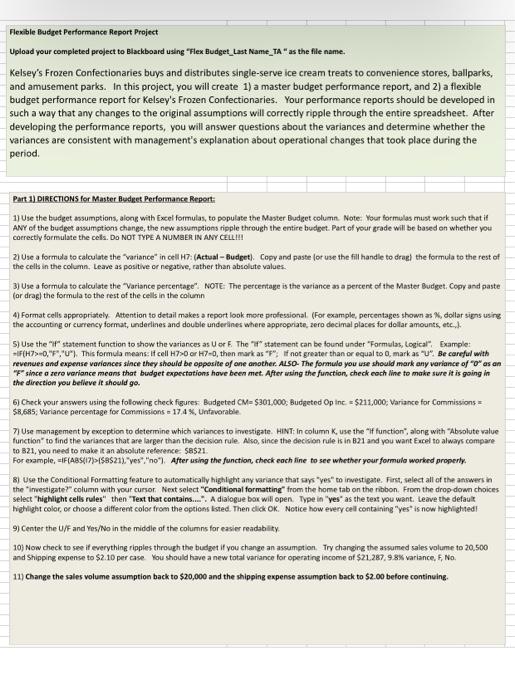
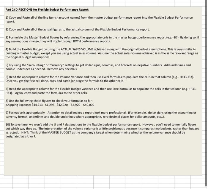
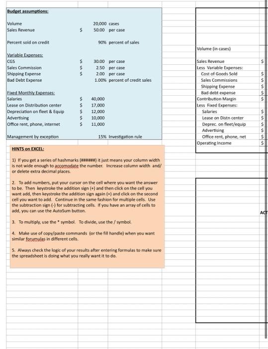
Flexible Budget Performance Report Project Upload your completed project to Blackboard using "Flex Budget_Last Name_TA" as the file name. Kelsey's Frozen Confectionaries buys and distributes single-serve ice cream treats to convenience stores, ballparks, and amusement parks. In this project, you will create 1) a master budget performance report, and 2) a flexible budget performance report for Kelsey's Frozen Confectionaries. Your performance reports should be developed in such a way that any changes to the original assumptions will correctly ripple through the entire spreadsheet. After developing the performance reports, you will answer questions about the variances and determine whether the variances are consistent with management's explanation about operational changes that took place during the period Part 1) DIRECTIONS for Master Budget Performance Report: 1) Use the budget assumptions, along with Excel formulas, to populate the Master Budget column. Note: Your formulas must work such that if ANY of the budget assumptions change, the new assumptions ripple through the entire budget. Part of your grade will be based on whether you correctly formulate the cells. Do NOT TYPE A NUMBER IN ANY CELIH 2) Use a formula to calculate the variance in cell H7. (Actual - Budget). Copy and paste for use the fill handle to drag the formula to the rest of the cells in the column Leave as positive or negative, rather than absolute values. JUse a formula to calculate the Variance percentage" NOTE: The percentage is the variance as a percent of the Master Budget. Copy and paste for drag the formula to the rest of the cells in the column 4) Format cells appropriately Attention to detail makes a report look more professional. (For example, percentages shown as dollar signs usine the accounting or currency format, underlines and double underines where appropriate, zero decimal places for dollar amounts, etc.. 5) Use the statement function to show the variances as U or 6 The statement can be found under "Formulas, Logical. Example: IF(H7>-0,"F","0"). This formula means:if cell H7>0 or H7-0, then mark as "F", if not greater than or equal to 0. mark as "U" Be careful with revenues and expense variances since they should be opposite of one another. ALSO. The formule you use should mark any variance of "o" as an since o zero variance means that budget expectations have been met. After wsing the function, check each line to make sure it is going in the direction you believe it should go. 6) Check your answers using the following check figures Badgeted CM= $301.000, Budgeted Op inc = $215,000; Variance for Commissions = $8,685, Variante percentage for Commissions - 17.4%. Unfavorable 7) Use management by exception to determine which variances to investigate. HINT: In column K use the function", along with "Absolute value function to find the variances that are larger than the decision rule Also, since the decision rule is in B21 and you want Excel to always compare to B21, you need to make it an absolute reference: 58$21. For example =IF[ABS(17)>$&$21. ves* "no"). After using the function, check each fine to see whether your formula worked properly. 8) Use the Conditional Formatting feature to automatically highlight any variance that says "yes" to investigate. First, select all of the answers in the investigate?" column with your cursor Next select "Conditional formatting from the home tab on the ribbon. From the drop down choices select "highlight cells rules" then "Text that contains.... A dialogue box wil open. Type in 'yes' as the text you want. Leave the default highlight color, or choose a different color from the options listed. Then dick OK. Notice how every cell containing "yes" is now highlighted 9) Center the U/F and Yes/No in the middle of the columns for easier readability 10) Now check to see if everything ripples through the budget If you change an assumption. Try changing the assumed sales volume to 20.500 and Shipping expense to $2.10 per case you should have a new total vanance for operating income of $21.287,98% variance, F, No. 11) Change the sales volume assumption back to $20,000 and the shipping expense assumption back to $2.00 before continuing Part 2) DIRECTIONS for Flexible Budget Performance Report: 1) Copy and paste all of the line items (account names) from the master budget performance report into the Flexible Budget Performance report. 2) Copy and paste all of the actual figures to the actual column of the Flexible Budget Performance report. 3) Formulate the Master Budget figures by referencing the appropriate cells in the master budget performance report (e.g.=B7). By doing so, if any assumptions change, they will ripple through BOTH performance reports. 4) Build the Flexible Budget by using the ACTUAL SALES VOLUME achieved along with the original budget assumptions. This is very similar to building a master budget, except you are using actual sales volume. Assume the actual sales volume achieved is in the same relevant range as the original budget assumptions. 5) Try using the "accounting" or "currency" settings to get dollar signs, commas, and brackets on negative numbers. Add underlines and double underlines as needed. Remove any decimals. 6) Head the appropriate column for the Volume Variance and then use Excel formulas to populate the cells in that column (e.g., +H33-33). Once you get the first cell done, copy and paste (or drag) the formula to the other cells. 7) Head the appropriate column for the Flexible Budget Variance and then use Excel formulas to populate the cells in that column (e.g. +F33- H33). Again, copy and paste the formulas to the other cells. 8) Use the following check figures to check your formulas so far: Shipping Expense: $44,213 $1,293 $42,920 $2,920 $40,000 9) Format cells appropriately. Attention to detail makes a report look more professional. (For example, dollar signs using the accounting or currency format, underlines and double underlines where appropriate, zero decimal places for dollar amounts, etc..). 10) To save time, we won't add the U and F designations to the flexible budget performance report. However, you'll need to mentally figure out which way they go. The interpretation of the volume variance is a little problematic because it compares two budgets, rather than budget vs. actual. HINT: Think of the MASTER BUDGET as the company's target when determining whether the volume variance should be designated as a U or F. Budget assumptions: Volume Sales Revenue 20.000 cases 50.00 per case $ Percent sold on credit 90% percent of sales Volume (in cases) $ Variable Fugenses CGS Sales Commission Shipping Expense Bad Debt Expense $ $ $ 30.00 per case 2.50 per case 2.00 per case 1.00% percent of credit sales $ s $ $ $ Sales Revenue Less Variable Expenses: Cost of Goods Sold Sales Commissions Shipping Expense Bad debt expense Contribution Margin Less Fixed Expenses: Salaries Lease on Distn center Deprec on fleet/equip Advertising Office rent, phone, net Operating Income $ $ $ $ $ $ Fbed Monthly Expenses: Salaries $ 40,000 Lease on Distribution center $ 17.000 Depreciation on fleet & Equip $ 12,000 Advertising $ 10,000 Office rent, phone, Internet $ 11,000 Management by exception 15% Investigation rule HINTS ON EXCEL 1) If you get a series of hashmarks () it just means your column width is not wide enough to accomodate the number. Increase column width and/ or delete extra decimal places. 2. To add numbers, put your cursor on the cell where you want the answer to be. Then keystroke the addition sign (+) and then click on the cell you want add, then keystroke the addition sign again (+) and click on the second cell you want to add. Continue in the same fashion for multiple cells. Use the subtraction sign (-) for subtracting cells. If you have an array of cells to add, you can use the AutoSum button 3. To multiply, use the symbol. To divide, use the symbol 4. Make use of copy/paste commands for the fill handie) when you want similar forumulas in different cells, 5 Always check the logic of your results after entering formulas to make sure the spreadsheet is doing what you really want it to do Kelsey's Frozen Confectionaries Master Budget Performance Report For the month ended June 30 MASTER BUDGET VARIANCE VAR.% For U Investigate? Volume (in cases) ACTUAL 21.460 $ 1,131,020 $ $ $ $ 682,880 58.685 44,213 16,930 328,312 Sales Revenue Less Variable Expenses: Cost of Goods Sold Sales Commissions Shipping Expense Bad debt expense Contribution Margin Less Fixed Expenses: Salaries Lease on Distn center Deprec. on fleet/equip Advertising Office rent, phone, net Operating income $ $ $ $ $ $ 43,000 15.500 12.000 7.750 12.300 237,762 Kelsey's Frozen Confectionaries Fexible Budget Performance Report For the month ended June 30 FLEXIBLE BUDGET ACTUAL MASTER BUDGET Flexible Budget Performance Report Project Upload your completed project to Blackboard using "Flex Budget_Last Name_TA" as the file name. Kelsey's Frozen Confectionaries buys and distributes single-serve ice cream treats to convenience stores, ballparks, and amusement parks. In this project, you will create 1) a master budget performance report, and 2) a flexible budget performance report for Kelsey's Frozen Confectionaries. Your performance reports should be developed in such a way that any changes to the original assumptions will correctly ripple through the entire spreadsheet. After developing the performance reports, you will answer questions about the variances and determine whether the variances are consistent with management's explanation about operational changes that took place during the period Part 1) DIRECTIONS for Master Budget Performance Report: 1) Use the budget assumptions, along with Excel formulas, to populate the Master Budget column. Note: Your formulas must work such that if ANY of the budget assumptions change, the new assumptions ripple through the entire budget. Part of your grade will be based on whether you correctly formulate the cells. Do NOT TYPE A NUMBER IN ANY CELIH 2) Use a formula to calculate the variance in cell H7. (Actual - Budget). Copy and paste for use the fill handle to drag the formula to the rest of the cells in the column Leave as positive or negative, rather than absolute values. JUse a formula to calculate the Variance percentage" NOTE: The percentage is the variance as a percent of the Master Budget. Copy and paste for drag the formula to the rest of the cells in the column 4) Format cells appropriately Attention to detail makes a report look more professional. (For example, percentages shown as dollar signs usine the accounting or currency format, underlines and double underines where appropriate, zero decimal places for dollar amounts, etc.. 5) Use the statement function to show the variances as U or 6 The statement can be found under "Formulas, Logical. Example: IF(H7>-0,"F","0"). This formula means:if cell H7>0 or H7-0, then mark as "F", if not greater than or equal to 0. mark as "U" Be careful with revenues and expense variances since they should be opposite of one another. ALSO. The formule you use should mark any variance of "o" as an since o zero variance means that budget expectations have been met. After wsing the function, check each line to make sure it is going in the direction you believe it should go. 6) Check your answers using the following check figures Badgeted CM= $301.000, Budgeted Op inc = $215,000; Variance for Commissions = $8,685, Variante percentage for Commissions - 17.4%. Unfavorable 7) Use management by exception to determine which variances to investigate. HINT: In column K use the function", along with "Absolute value function to find the variances that are larger than the decision rule Also, since the decision rule is in B21 and you want Excel to always compare to B21, you need to make it an absolute reference: 58$21. For example =IF[ABS(17)>$&$21. ves* "no"). After using the function, check each fine to see whether your formula worked properly. 8) Use the Conditional Formatting feature to automatically highlight any variance that says "yes" to investigate. First, select all of the answers in the investigate?" column with your cursor Next select "Conditional formatting from the home tab on the ribbon. From the drop down choices select "highlight cells rules" then "Text that contains.... A dialogue box wil open. Type in 'yes' as the text you want. Leave the default highlight color, or choose a different color from the options listed. Then dick OK. Notice how every cell containing "yes" is now highlighted 9) Center the U/F and Yes/No in the middle of the columns for easier readability 10) Now check to see if everything ripples through the budget If you change an assumption. Try changing the assumed sales volume to 20.500 and Shipping expense to $2.10 per case you should have a new total vanance for operating income of $21.287,98% variance, F, No. 11) Change the sales volume assumption back to $20,000 and the shipping expense assumption back to $2.00 before continuing Part 2) DIRECTIONS for Flexible Budget Performance Report: 1) Copy and paste all of the line items (account names) from the master budget performance report into the Flexible Budget Performance report. 2) Copy and paste all of the actual figures to the actual column of the Flexible Budget Performance report. 3) Formulate the Master Budget figures by referencing the appropriate cells in the master budget performance report (e.g.=B7). By doing so, if any assumptions change, they will ripple through BOTH performance reports. 4) Build the Flexible Budget by using the ACTUAL SALES VOLUME achieved along with the original budget assumptions. This is very similar to building a master budget, except you are using actual sales volume. Assume the actual sales volume achieved is in the same relevant range as the original budget assumptions. 5) Try using the "accounting" or "currency" settings to get dollar signs, commas, and brackets on negative numbers. Add underlines and double underlines as needed. Remove any decimals. 6) Head the appropriate column for the Volume Variance and then use Excel formulas to populate the cells in that column (e.g., +H33-33). Once you get the first cell done, copy and paste (or drag) the formula to the other cells. 7) Head the appropriate column for the Flexible Budget Variance and then use Excel formulas to populate the cells in that column (e.g. +F33- H33). Again, copy and paste the formulas to the other cells. 8) Use the following check figures to check your formulas so far: Shipping Expense: $44,213 $1,293 $42,920 $2,920 $40,000 9) Format cells appropriately. Attention to detail makes a report look more professional. (For example, dollar signs using the accounting or currency format, underlines and double underlines where appropriate, zero decimal places for dollar amounts, etc..). 10) To save time, we won't add the U and F designations to the flexible budget performance report. However, you'll need to mentally figure out which way they go. The interpretation of the volume variance is a little problematic because it compares two budgets, rather than budget vs. actual. HINT: Think of the MASTER BUDGET as the company's target when determining whether the volume variance should be designated as a U or F. Budget assumptions: Volume Sales Revenue 20.000 cases 50.00 per case $ Percent sold on credit 90% percent of sales Volume (in cases) $ Variable Fugenses CGS Sales Commission Shipping Expense Bad Debt Expense $ $ $ 30.00 per case 2.50 per case 2.00 per case 1.00% percent of credit sales $ s $ $ $ Sales Revenue Less Variable Expenses: Cost of Goods Sold Sales Commissions Shipping Expense Bad debt expense Contribution Margin Less Fixed Expenses: Salaries Lease on Distn center Deprec on fleet/equip Advertising Office rent, phone, net Operating Income $ $ $ $ $ $ Fbed Monthly Expenses: Salaries $ 40,000 Lease on Distribution center $ 17.000 Depreciation on fleet & Equip $ 12,000 Advertising $ 10,000 Office rent, phone, Internet $ 11,000 Management by exception 15% Investigation rule HINTS ON EXCEL 1) If you get a series of hashmarks () it just means your column width is not wide enough to accomodate the number. Increase column width and/ or delete extra decimal places. 2. To add numbers, put your cursor on the cell where you want the answer to be. Then keystroke the addition sign (+) and then click on the cell you want add, then keystroke the addition sign again (+) and click on the second cell you want to add. Continue in the same fashion for multiple cells. Use the subtraction sign (-) for subtracting cells. If you have an array of cells to add, you can use the AutoSum button 3. To multiply, use the symbol. To divide, use the symbol 4. Make use of copy/paste commands for the fill handie) when you want similar forumulas in different cells, 5 Always check the logic of your results after entering formulas to make sure the spreadsheet is doing what you really want it to do Kelsey's Frozen Confectionaries Master Budget Performance Report For the month ended June 30 MASTER BUDGET VARIANCE VAR.% For U Investigate? Volume (in cases) ACTUAL 21.460 $ 1,131,020 $ $ $ $ 682,880 58.685 44,213 16,930 328,312 Sales Revenue Less Variable Expenses: Cost of Goods Sold Sales Commissions Shipping Expense Bad debt expense Contribution Margin Less Fixed Expenses: Salaries Lease on Distn center Deprec. on fleet/equip Advertising Office rent, phone, net Operating income $ $ $ $ $ $ 43,000 15.500 12.000 7.750 12.300 237,762 Kelsey's Frozen Confectionaries Fexible Budget Performance Report For the month ended June 30 FLEXIBLE BUDGET ACTUAL MASTER BUDGET