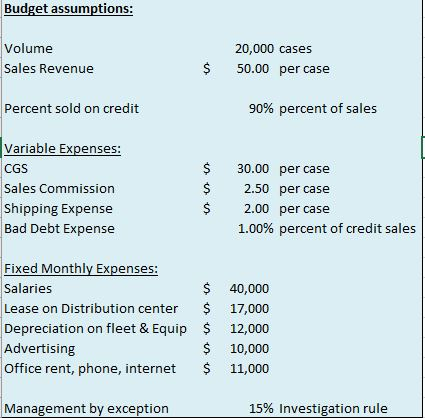
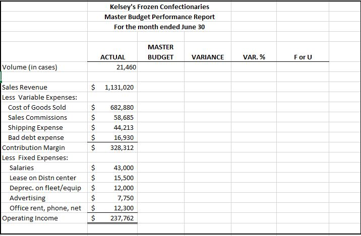
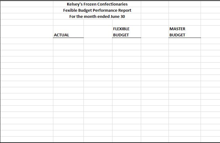
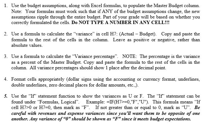
Please show work in excel Budget assumptions: Volume Sales Revenue 20,000 cases 50.00 per case $ Percent sold on credit 90% percent of sales Variable Expenses: CGS Sales Commission Shipping Expense Bad Debt Expense $ $ 30.00 per case 2.50 per case 2.00 per case 1.00% percent of credit sales Fixed Monthly Expenses: Salaries Lease on Distribution center Depreciation on fleet & Equip Advertising Office rent, phone, internet $ $ $ $ $ 40,000 17,000 12,000 10,000 11,000 Management by exception 15% Investigation rule Kelsey's Frozen Confectionaries Master Budget Performance Report For the month ended June 30 MASTER BUDGET VARIANCE VAR.% For U ACTUAL 21,460 Volume (in cases) $ 1,131,020 $ $ $ $ 682,880 58,685 44,213 16,930 328,312 Sales Revenue Less Variable Expenses: Cost of Goods Sold Sales Commissions Shipping Expense Bad debt expense Contribution Margin Less Fixed Expenses: Salaries Lease on Distn center Deprec. on fleet/equip Advertising Office rent, phone, net Operating Income $ $ 43,000 15,500 12,000 7,750 12,300 237,762 $ $ Kelsey's Frozen Confectionaries Fexible Budget Performance Report For the month ended June 30 FLEXIBLE BUDGET MASTER BUDGET ACTUAL 1. Use the budget assumptions, along with Excel formulas, to populate the Master Budget column. Note: Your formulas must work such that if ANY of the budget assumptions change, the new assumptions ripple through the entire budget. Part of your grade will be based on whether you correctly formulated the cells. Do NOT TYPE A NUMBER IN ANY CELL!!! 2. Use a formula to calculate the "variance in cell H7: (Actual - Budget). Copy and paste the formula to the rest of the cells in the column. Leave as positive or negative, rather than absolute values. 3. Use a formula to calculate the "Variance percentage". NOTE: The percentage is the variance as a percent of the Master Budget. Copy and paste the formula to the rest of the cells in the column. All variance percentages should show 1 place after the decimal point. 4. Format cells appropriately (dollar signs using the accounting or currency format, underlines, double underlines, zero decimal places for dollar amounts, etc.). 5. Use the "If statement function to show the variances as U or F. The "If statement can be found under "Formulas, Logical". Example: =IF(H7>=0."F","U"). This formula means "If cell H7>0 or H7=0, then mark as "F". If not greater than or equal to 0. mark as U. Be careful with revenues and expense variances since you'll want them to be opposite of one another. Any variance of "0" should be shown as "F" since it meets budget expectations