Please solve Questions 1-5. Vlab part 1 questions v25

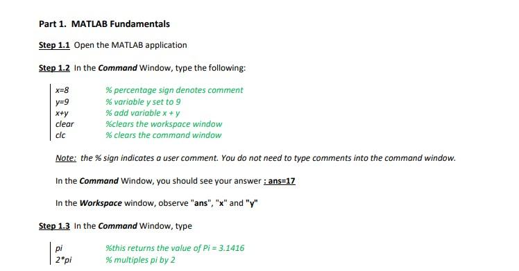
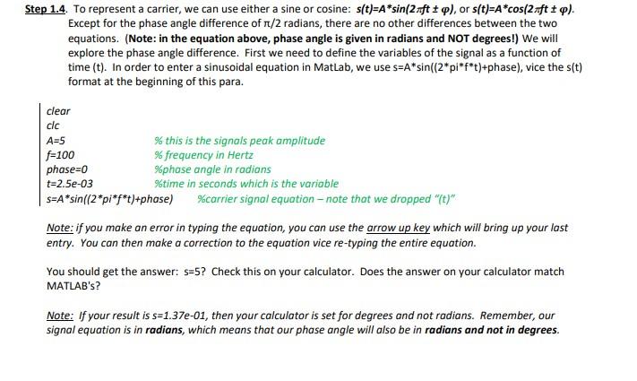
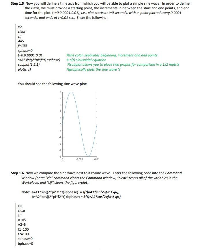
Part 1. MATLAB Fundamentals Step 1.1 Open the MATLAB application Step 1.2 In the Command Window, type the following: Note: the % sign indicates a user comment. You do not need to type comments into the command window. In the Command Window, you should see your answer : ans=17 In the Workspace window, observe "ans", " x " and " y " Step 1.3 In the Command Window, type pi2pi%thisreturnsthevalueofPi=3.1416%multiplespiby2 Step 1.4. To represent a carrier, we can use either a sine or cosine: s(t)=Asin(2ft), or s(t)=Acos(2ft). Except for the phase angle difference of /2 radians, there are no other differences between the two equations. (Note: in the equation above, phase angle is given in radians and NOT degrees!) We will explore the phase angle difference. First we need to define the variables of the signal as a function of time (t). In order to enter a sinusoidal equation in MatLab, we use s=Asin((2pift)+ phase), vice the s(t) format at the beginning of this para. Note: if you make an error in typing the equation, you can use the arrow up key which will bring up your last entry. You can then make a correction to the equation vice re-typing the entire equation. You should get the answer: s=5 ? Check this on your calculator. Does the answer on your calculator match MATLAB's? Note: If your result is s=1.37e01, then your calculator is set for degrees and not radians. Remember, our signal equation is in radians, which means that our phase angle will also be in radians and not in degrees. Step 1.5 Now you will define a time axis from which you will be able to plot a simple sine wave. In order to define the x axis, we must provide a starting point, the increments in-between the start and end points, and end time for the plot (t=0:0.0001:0.01); i.e., plot starts at t=0 seconds, with a point plotted every 0.0001 seconds, and ends at t=0.01sec. Enter the following: You should see the following sine wave plot: Step 1.6 Now we compare the sine wave next to a cosine wave. Enter the following code into the Command Window (note: "clc" command clears the Command window, "clear" resets all of the variables in the Workplace, and "clf" clears the figure/plot). Note: s=A1sin((2piif1t)+sshhse)=s(t)=A1sin(2f1ts), b=A2cos((2pif2t)+bphase)=b(t)=A2cos(2f2tb), clcclearclfA1=5A2=5f1=100f2=100sphase=0bphase=0 We see that the cosine wave on the right appears as a sine wave that has shifted 90 degrees to the left. Another way to interpret this is by saying that the cosine wave, since it has a peak amplitude earlier than the sine wave, "leads" the sine wave by 90 degrees or +1.57 radians. Step 1.7 Now let's shift the cosine wave form, "b", by -pi/2 radians. You should see that both s(t) and b(t) appear the same - i.e., both look like sine waves. Since the cosine wave had to shift -90 degrees in phase in order to look like the sine wave, we can say that the cosine wave "leads" the sine wave by 90 degrees. We can also say that the sine wave "lags" the cosine wave by 90 degrees. Step 1.8 Next, we change some variables and plot the resulting sinusoids onto a single plot in order to better see the differences between the sinusoids. Note: variables are changed directly into the script! (1) s(t)=s=A1sin((2 pi*f1*t )+sphase)=3sin(2150t+0),A1=3,f1=150, sphase =0 (2) b(t)=b=A2cos((2pif2t)+bphase)=5cos(2150t+0),A2=5,f2=150, bphase =0 The cosine plot leads the sine plot by /2 radians. In addition, the cosine wave has an amplitude of 5 volts compared to the sine wave amplitude of 3 volts. (1) s(t)=s=A1sin((2pif1t)+sphase)=5sin(2500t+0) (2) b(t)=b=A2cos((2pif2t)+bphase)=2cos(2500t/2) Question 1. Select the best answer regarding your observation from step 1.9. a. both s(t) and b(t) appear as identical sine waves in frequency, amplitude, and phase b. both s(t) and b(t) are at the same frequency but with different amplitudes c. the frequency of s(t) is higher than the frequency of b(t) d. both s(t) and b(t) differ in frequency and amplitude Plot 1 - Sine Cosine Wave Plot Submission: Submit (i.e., copy/paste) the MATLAB plots from step 1.9 above into the "IT300 Virtual Lab Plot Submission" document template. Note: After executing the plot command, go to the plot and perform a "copy figure" under the "Edit" menu. Paste this figure into the assignment "IT300 Virtual Lab Plot Submission" on Bb Assignments/Virtual LAB folder. Step 1.10 Now plot the following carrier waves s(t) and b(t). Place both plots onto a single graph as you did in steps 1.8 and 1.9. (1) s(t)=s=A1sin((2pif1t)+sphase)=3sin(2350t+0) (2) b(t)=b=A2cos((2pif2t)+bphase)=3cos(2250t+0) Question 2. What are the differences between the two plots s(t) and b(t) from step 1.10? a. s(t) and b(t) have the same frequencies b. s(t) and b(t) have same amplitudes c. s(t) and b(t) differ in amplitude and frequency d. all of the above are correct Plot 2 - Sine Cosine Wave Plot Submission: Submit (i.e., copy/paste) the MATLAB plots from step 1.10 above into the "IT300 Virtual Lab Plot Submission". Step 1.11 Plot s(t) and b(t) in a single plot. (1) s(t)=s=A1sin((2 pi*f1*t )+sphase)=4sin(2300t+0) (2) b(t)=b=A2cos((2pif2t)+bphase)=4cos(2300t/2) Question 3 Select the correct observation for s(t) and b(t) a. plots are same in amplitude but differ in frequency b. plots appear to differ in amplitude c. plots appear as distinct cosine and sine waves at t=0 d. both plots appear as identical waves Plot 3 - Sine Cosine Wave Plot Submission: Submit (i.e., copy/paste) the MATLAB plots from step 1.11 above into the "IT300 Virtual Lab Plot Submission". Part 2. Amplitude Modulation message or modulating signal: carrier: modulation index: AM modulation formula: s(t)=Ac[1+cos(2fmt)]cos(2fct),s=s=Ac(1+micos(2pifmt))cos(2pift),MatLabform tep 2.1 Plot the following equations: m(t)=3cos(21700Hzt)c(t)=5cos(210.5kHzt) NOTE: when you save your MATLAB file, the name of your file cannot contain spaces. An example of a legal file name is "LAB_IT300_step23" \%AM Modulation; clear; clc; clf; Ac=5; Am=3; fc=10500; fm=1700; t=0:0.00001:0.003; m=Am*cos(2*pi*fm*t); c=Ac*cos(2*pi*fc*t); mi = Am/Ac; s=Ac*(1+mi*cos(2*pi*fm**t)).* cos(2 pi*fe*t); subplot(2,2,1); plot(t,s); xlabel('time'); ylabel('amplitude'); title('AM modulation'); subplot(2,2,4); plot(t,m); xlabel('time'); ylabel('amplitude'); title('Message'); subplot(2,2,2); plot (t,c); xlabel('time'); ylabel('amplitude'); title('Carrier'); subplot(2,2,3); yyaxis left; plot(t,m); ylim([-10 10]) yyaxis right; plot(t,s); ylim([-10 10]) title('combined message and signal'); You Figure 1 plot fo chan\& wave. m(t)=2cos(2500Hzt)c(t)=5cos(29kzt) Question 4. Having made the changes, select the correct statement regarding your observation. a. The signal, s(t), faithfully represents the original message wave m(t) b. The receiver will be unable to demodulate the modulated carrier wave shown in the upper left plot c. The AM modulated carrier shows significant signal distortion d. a and b Plot 4 - AM Signal Plot Submission: Submit (i.e., copy/paste) the MATLAB plots from step 2.2 above into the "IT300 Virtual Lab Plot Submission". Step 2.3 Plot the following equations: m(t)=12cos(2500Hzt)c(t)=5cos(210kHzt) Question 5. Select the correct statement that describes what you see in the plots: a. The signal, s(t), is distorted because the AM Index value is too high 9 b. The modulated signal accurately represents m(t) c. Distortion is experienced because the message and carrier frequencies are too far apart from one another d. The phase of the signal has shifted to the right because AM techniques impact phase and amplitude. Plot 5 - AM Signal Plot Submission: Submit (i.e., copy/paste) the MATLAB plots from step 2.3 above into the "IT300 Virtual Lab Plot Submission v13