Please solve this Excel spreadsheet using the directions! Thank you so much!

Directions:

Excel Spreadsheet:

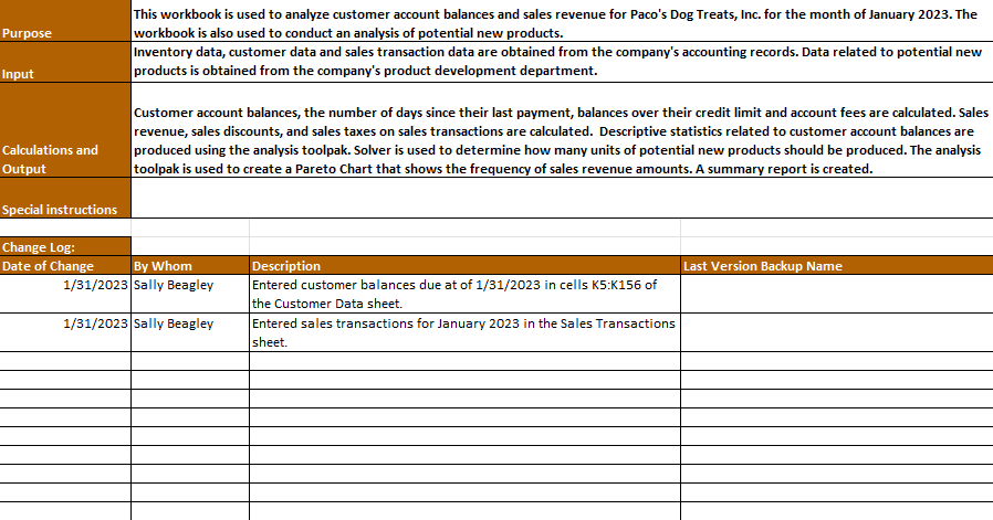
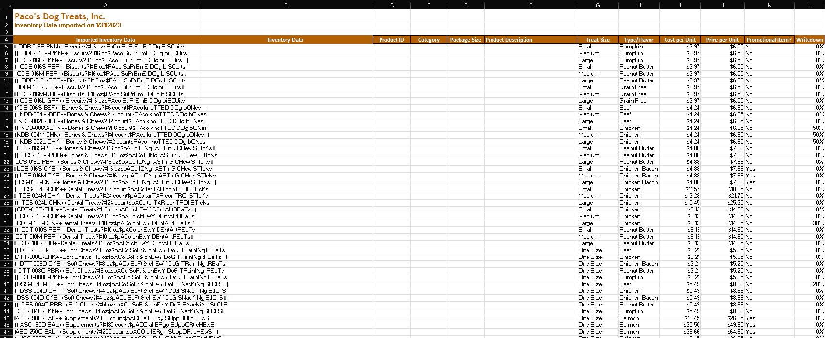
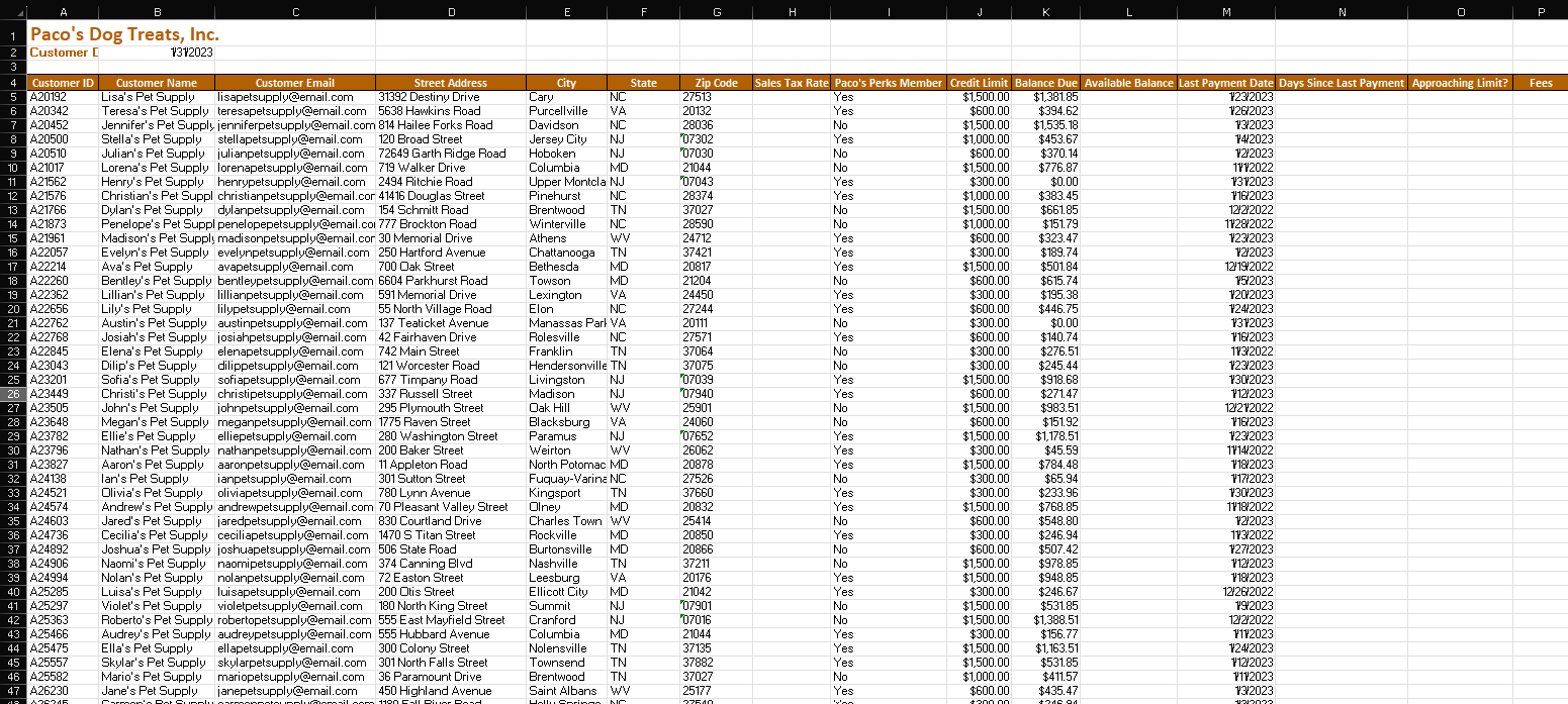
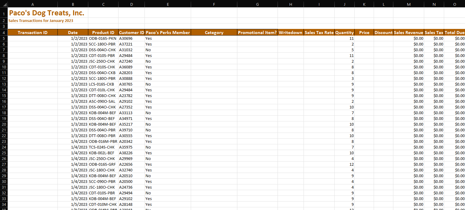
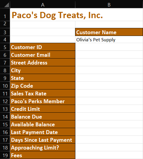
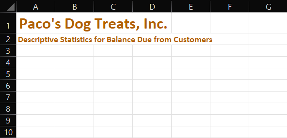
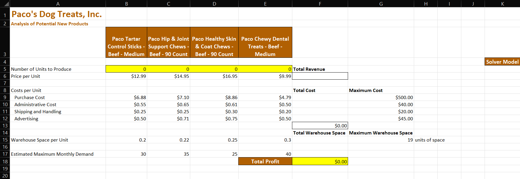
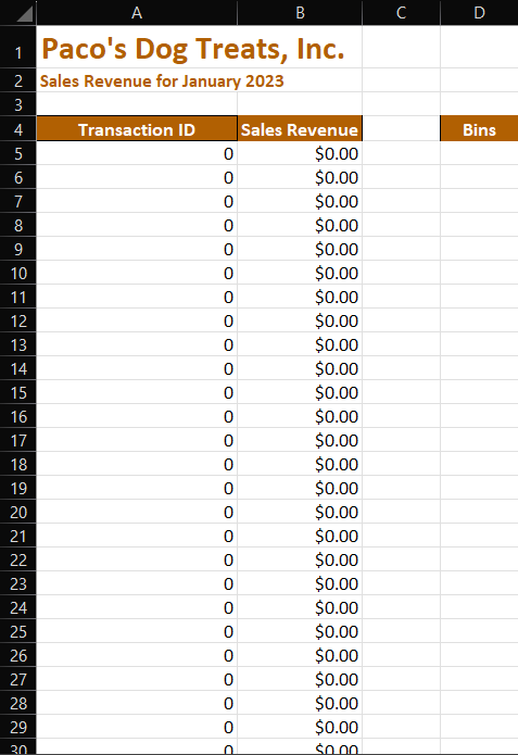
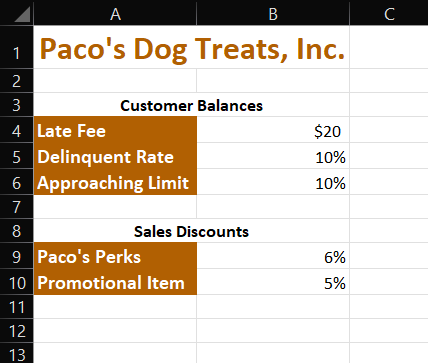
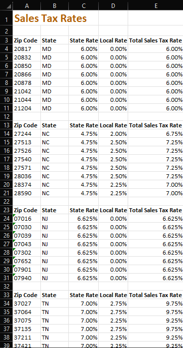
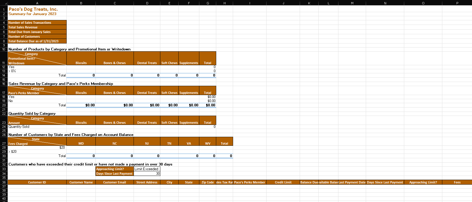
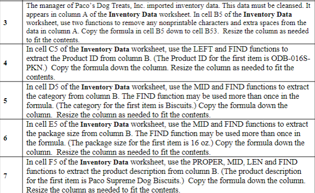
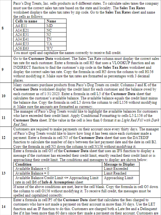
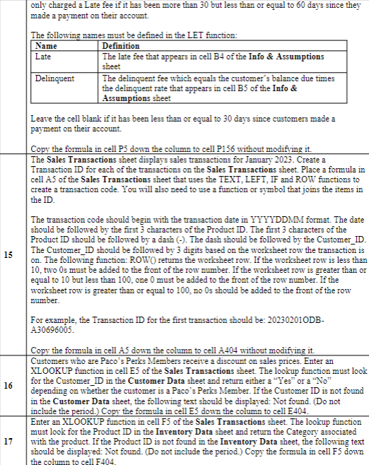
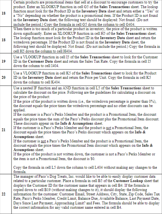
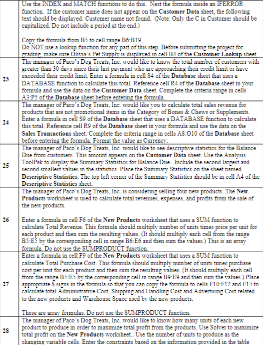
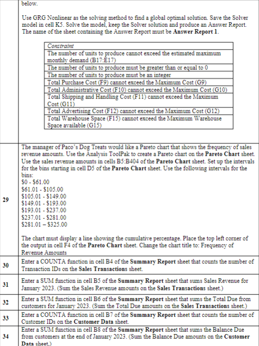
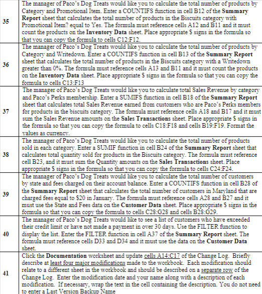
The manager of Paco's Dog Treats, Inc. imported inventory data. This data must be cleansed. It appears in column A of the Inventory Data worksheet. In cell B 5 of the Inventory Data worksheet, use two functions to remove any nonprintable characters and extra spaces from the data in column A. Copy the formula in cell B5 down to cell B53. Resize the column as needed to fit the contents. In cell C5 of the Inventory Data worksheet, use the LEFT and FIND functions to extract the Product ID from column B. (The Product ID for the first item is ODB-016SPKN.) Copy the formula down the column. Resize the column as needed to fit the contents. In cell D5 of the Inventory Data worksheet, use the MID and FIND functions to extract the category from column B. The FIND function may be used more than once in the formula. (The category for the first item is Biscuits.) Copy the formula down the column. Resize the column as needed to fit the contents. In cell E5 of the Inventory Data worksheet, use the MID and FIND functions to extract the package size from column B. The FIND function may be used more than once in the formula. (The package size for the first item is 16oz.) Copy the formula down the column. Resize the column as needed to fit the contents. In cell F5 of the Inventory Data worksheet, use the PROPER, MID, LEN and FIND functions to extract the product description from column B. (The product description for the first item is Paco Supreme Dog Biscuits.) Copy the formula down the column. Resize the column as needed to fit the contents. Paco's Dog Treats, Inc. sells products in 6 different states. To calculate sales taxes the company must use the correct sales tax rate based on the state and locality. The Sales Tax Rates worksheet displays the sales tax rates by zip code. Go to the Sales Tax Rates sheet and name the cells as follows: only charged a Late fee if it has been more than 30 but less than or equal to 60 days since they made a payment on their account. The followine names murt he defined in the T FT finction- Leave the cell blank if it has been less than or equal to 30 days since customers made a payment on their account. Copv the formula in cell P5 down the column to cell P156 without modifving it. The Sales Transactions sheet displays sales transactions for January 2023. Create a Transaction ID for each of the transactions on the Sales Transactions sheet. Place a formula in cell A.5 of the Sales Transactions sheet that uses the TEXT, LEFT, IF and ROW functions to create a transaction code. You will also need to use a function or symbol that joins the items in the ID. The transaction code should begin with the transaction date in YYYYDDMM format. The date should be followed by the first 3 characters of the Product ID. The first 3 characters of the Product ID should be followed by a dash (). The dash should be followed by the Customer_ID. The Customer_ID should be followed by 3 digits based on the worksheet row the transaction is on. The following function: ROWO retums the worksheet row. If the worksheet row is less than 10 , two 0 s must be added to the front of the row number. If the worksheet row is greater than or equal to 10 but less than 100 , one 0 must be added to the front of the row number. If the worksheet row is greater than or equal to 100 , no 0 s should be added to the front of the row number. For example, the Transaction ID for the first transaction should be: 202302010DBA.30696005. Copy the formula in cell A.5 down the column to cell A404 without modifving it. Customers who are Paco's Perks Members receive a discount on sales prices. Enter an XLOOKUP function in cell E5 of the Sales Transactions sheet. The lookup function must look for the Customer_ID in the Customer Data sheet and return either a "Yes" or a "No" depending on whether the customer is a Paco's Perks Member. If the Customer ID is not found in the Customer Data sheet, the following text should be displayed: Not found. (Do not include the period.) Copv the formula in cell E5 down the column to cell E404. Enter an XLOOKUP function in cell F5 of the Sales Transactions sheet. The lookup function must look for the Product ID in the Inventory Data sheet and return the Category associated with the product. If the Product ID is not found in the Inventory Data sheet, the following text should be displayed: Not found. (Do not include the period.) Copy the formula in cell F5 down the column to cell F404. Certain products are promotional items that sell at a discount to encourage customers to try the product. Enter an XLOOKUP function in cell G5 of the Sales Transactions sheet. The lookup function must look for the Product ID in the Inventory Data sheet and return either a "Yes" or a "No" depending on whether the product is a promotional item. If the Product ID is not found in the Inventory Data sheet, the following text should be displayed: Not found. (Do not include the period.) Copv the formula in cell G5 down the column to cell G404. When there is too much of a particular product in inventory, the price of the product is written down significantly. Enter an XLOOKUP function in cell H5 of the Sales Transactions sheet. The lookup function must look for the Product ID in the Inventory Data sheet and return the writedown percentage. If the Product ID is not found in the Inventory Data sheet, the following text should be displayed: Not found. (Do not include the period.) Copy the formula in cell H5 down the column to cell H404. Use a VLOOKUP function in cell I5 of the Sales Transactions sheet to look for the Customer ID in the Customer Data sheet and retum the Sales Tax Rate. Copy the formula in cell I5 down the column to cell 1404 . Use a VLOOKUP function in cell K5 of the Sales Transactions sheet to look for the Product ID in the Inventory Data sheet and retum the Price per Unit. Copy the formula in cell K 5 down the column to cell K404. Use a nested IF function and an AND function in cell L5 of the Sales Transactions sheet to calculate the discount on the price. Following are the guidelines for calculating a discount on the price of the product: If the price of the product is written down (i.e., the writedown percentage is greater than 0% ), the discount equals the price times the writedown percentage and no other discounts can be applied. If the customer is a Paco's Perks Member and the product is a Promotional Item, the discount equals the price times the sum of the Paco's Perks discount plus the Promotional Item discount. These discounts appear on the Info \& Assumptions sheet. If the customer is a Paco's Perks Member and the product is not a Promotional Item, the discount equals the price times the Paco's Perks discount which appears on the Info \& Assumptions sheet. If the customer is not a Paco's Perks Member and the product is a Promotional Item, the discount equals the price times the Promotional Item discount which appears on the Info \& Assumptions sheet. If the price of the product is not written down, the customer is not a Paco's Perks Member or the item is not a Promotional ltem, the discount is $0. Copy the formula in cell L5 down the column to cell L404 without making any changes to the formula. The manager of Paco's Dog Treats, Inc. would like to be able to easily display customer data related to a particular customer. Place a formula in cell B5 of the Customer Lookup sheet that displays the Customer ID for the customer name that appears in cell B4. If the formula is copied down to cell B19 (without making changes to it), it should display the following information for the customer: Customer Email, Street Address, City, State, Zip Code, Sales Tax Rate, Paco's Perks Member, Credit Limit, Balance Due, Available Balance, Last Payment Date, Days Since Last Payment, Approaching Limit? and Fees. The formula should be able to display the correct information for any valid customer name entered in cell B4. Use the INDEX and MATCH functions to do this. Nest the formula inside an IFERROR function. If the customer name does not appear on the Customer Data sheet, the following text should be displayed: Customer name not found. (Note: Only the C in Customer should be capitalized. Do not include a period at the end.) Copy the formula from B5 to cell range B6:B19. Do NOT use a lookup function for any part of this step. Before submitting the project for grading. make sure Olivia's Pet Supply is displayed in cell B4 of the Customer Lookup sheet. The manager of Paco's Dog Treats, Inc. would like to know the total number of customers with greater than 30 days since their last payment who are approaching their credit limit or have exceeded their credit limit. Enter a formula in cell S4 of the Database sheet that uses a DATABASE function to calculate this total. Reference cell R4 of the Database sheet in your formula and use the data on the Customer Data sheet. Complete the criteria range in cells A.3:P5 of the Database sheet before entering the formula. The manager of Paco's Dog Treats, Inc. would like you to calculate total sales revenue for products that are not promotional items in the Category of Bones \& Chews or Supplements. Enter a formula in cell S9 of the Database sheet that uses a DATABASE function to calculate this total. Reference cell Rg of the Database sheet in your formula and use the data on the Sales Transactions sheet. Complete the criteria range in cells A8:010 of the Database sheet before entering the formula. Format the value as Currency. The manager of Paco's Dog Treats, Inc. would like to see descriptive statistics for the Balance Due from customers. This amount appears on the Customer Data sheet. Use the Analysis ToolPak to display the Summary Statistics for Balance Due. Include the second largest and second smallest values in the statistics. Place the Summary Statistics on the sheet named Descriptive Statistics. The top left comer of the Summary Statistics should be in cell A4 of the Descriptive Statistics sheet. The manager of Paco's Dog Treats, Inc. is considering selling four new products. The New Products worksheet is used to calculate total revenues, expenses, and profits from the sale of the new products. Enter a formula in cell F6 of the New Products worksheet that uses a SUM function to calculate Total Revenue. This formula should multiply number of units times price per unit for each product and then sum the resulting values. (It should multiply each cell from the range B5:E5 by the corresponding cell in range B6:E6 and then sum the values.) This is an array formula. Do not use the SUMPRODUCT function. Enter a formula in cell F9 of the New Products worksheet that uses a SUM function to calculate Total Purchase Cost. This formula should multiply number of units times purchase cost per unit for each product and then sum the resulting values. (It should multiply each cell from the range B5:E5 by the corresponding cell in range B9E9 and then sum the values.) Place appropriate S signs in the formula so that you can copy the formula to cells F10:F12 and F15 to calculate total Administrative Cost, Shipping and Handling Cost and Advertising Cost related to the new products and Warehouse Space used by the new products. These are array formulas. Do not use the SUMPRODUCT function. The manager of Paco's Dog Treats, Inc. would like to know how many units of each new product to produce in order to maximize total profit from the products. Use Solver to maximize total profit on the New Products worksheet. Use the number of units to produce as the changing variable cells. Enter the constraints based on the information provided in the table below. Use GRG Nonlinear as the solving method to find a global optimal solution. Save the Solver model in cell K5. Solve the model, keep the Solver solution and produce an Answer Report. The name of the sheet containing the Answer Report must be Answer Report 1. The manager of Paco's Dog Treats would like a Pareto chart that shows the frequency of sales revenue amounts. Use the Analysis ToolPak to create a Pareto chart on the Pareto Chart sheet. Use the sales revenue amounts in cells B5:B404 of the Pareto Chart sheet. Set up the intervals for the bins starting in cell D5 of the Pareto Chart sheet. Use the following intervals for the bins: $0$61.00 $61.01$105.00 $105.01$149.00 $149.01$193.00 $193.01$237.00 $237.01$281.00 $281.01$325.00 The chart must display a line showing the cumulative percentage. Place the top left corner of the output in cell F4 of the Pareto Chart sheet. Change the chart title to: Frequency of The manager of Paco's Dog Treats would like you to calculate the total number of products by Category and Promotional Item. Enter a COUNTIFS function in cell B12 of the Summary Report sheet that calculates the total number of products in the Biscuits category with Promotional Item? equal to Yes. The formula must reference cells A12 and B11 and it must count the products on the Inventory Data sheet. Place appropriate $ signs in the formula so that you can copv the formula to cells C12F12. The manager of Paco's Dog Treats would like you to calculate the total number of products by Category and Writedown. Enter a COUNTIFS function in cell B13 of the Summary Report sheet that calculates the total number of products in the Biscuits category with a Writedown greater than 0%. The formula must reference cells A 13 and B11 and it must count the products on the Inventory Data sheet. Place appropriate $ signs in the formula so that you can copy the formula to cells C13 :F13 The manager of Paco's Dog Treats would like you to calculate total Sales Revenue by category and Paco's Perks membership. Enter a SUMIFS function in cell B18 of the Summary Report sheet that calculates total Sales Revenue eamed from customers who are Paco's Perks members for products in the biscuits category. The formula must reference cells A18 and B17 and it must sum the Sales Revenue amounts on the Sales Transactions sheet. Place appropriate $ signs in the formula so that you can copy the formula to cells C18-F18 and cells B19-F19. Format the values as currency. The manager of Paco's Dog Treats would like you to calculate the total number of products sold in each category. Enter a SUMIF function in cell B24 of the Summary Report sheet that calculates total quantity sold for products in the Biscuits category. The formula must reference cell B23, and it must sum the Quantity amounts on the Sales Transactions sheet. Place appropriate S signs in the formula so that you can copy the formula to cells C24:F24. The manager of Paco3 Dog Treats would like you to calculate the total number of customers by state and fees charged on their account balance. Enter a COUNTIFS function in cell B28 of the Summary Report sheet that calculates the total number of customers in Maryland that are charged fees equal to $20 in January. The formula must reference cells A.28 and B27 and it must use the State and Fees data on the Customer Data sheet. Place appropriate S signs in the formula so that you can copy the formula to cells C28:G28 and cells B28:G29. The manager of Paco's Dog Treats would like to see a list of customers who have exceeded their credit limit or have not made a payment in over 30 days. Use the FIL TER function to display the list. Enter the FILTER. function in cell A.37 of the Summary Report sheet. The formula must reference cells D33 and D34 and it must use the data on the Customer Data sheet. Click the Documentation worksheet and update cells A14:C17 of the Change Log. Briefly describe at least four major modifications made to the workbook. Each modification should relate to a different sheet in the workbook and should be described on a separate row of the Change Log. Enter the modification date and your name along with a description of each modification. If necessary, wrap the text in the cell containing the description. You do not need to enter a Last Version Backup Name This workbook is used to analyze customer account balances and sales revenue for Paco's Dog Treats, Inc. for the month of January 2023 . The workbook is also used to conduct an analysis of potential new products. Inventory data, customer data and sales transaction data are obtained from the company's accounting records. Data related to potential new products is obtained from the company's product development department. Customer account balances, the number of days since their last payment, balances over their credit limit and account fees are calculated. Sales revenue, sales discounts, and sales taxes on sales transactions are calculated. Descriptive statistics related to customer account balances are Calculations and produced using the analysis toolpak. Solver is used to determine how many units of potential new products should be produced. The analysis Output toolpak is used to create a Pareto Chart that shows the frequency of sales revenue amounts. A summary report is created. Special instructions Change Log: Paco's Dog Treats, Inc. A B 412345678910 Paco's Dog Treats, Inc. Descriptive Statistics for Balance Due from Customers The manager of Paco's Dog Treats, Inc. imported inventory data. This data must be cleansed. It appears in column A of the Inventory Data worksheet. In cell B 5 of the Inventory Data worksheet, use two functions to remove any nonprintable characters and extra spaces from the data in column A. Copy the formula in cell B5 down to cell B53. Resize the column as needed to fit the contents. In cell C5 of the Inventory Data worksheet, use the LEFT and FIND functions to extract the Product ID from column B. (The Product ID for the first item is ODB-016SPKN.) Copy the formula down the column. Resize the column as needed to fit the contents. In cell D5 of the Inventory Data worksheet, use the MID and FIND functions to extract the category from column B. The FIND function may be used more than once in the formula. (The category for the first item is Biscuits.) Copy the formula down the column. Resize the column as needed to fit the contents. In cell E5 of the Inventory Data worksheet, use the MID and FIND functions to extract the package size from column B. The FIND function may be used more than once in the formula. (The package size for the first item is 16oz.) Copy the formula down the column. Resize the column as needed to fit the contents. In cell F5 of the Inventory Data worksheet, use the PROPER, MID, LEN and FIND functions to extract the product description from column B. (The product description for the first item is Paco Supreme Dog Biscuits.) Copy the formula down the column. Resize the column as needed to fit the contents. Paco's Dog Treats, Inc. sells products in 6 different states. To calculate sales taxes the company must use the correct sales tax rate based on the state and locality. The Sales Tax Rates worksheet displays the sales tax rates by zip code. Go to the Sales Tax Rates sheet and name the cells as follows: only charged a Late fee if it has been more than 30 but less than or equal to 60 days since they made a payment on their account. The followine names murt he defined in the T FT finction- Leave the cell blank if it has been less than or equal to 30 days since customers made a payment on their account. Copv the formula in cell P5 down the column to cell P156 without modifving it. The Sales Transactions sheet displays sales transactions for January 2023. Create a Transaction ID for each of the transactions on the Sales Transactions sheet. Place a formula in cell A.5 of the Sales Transactions sheet that uses the TEXT, LEFT, IF and ROW functions to create a transaction code. You will also need to use a function or symbol that joins the items in the ID. The transaction code should begin with the transaction date in YYYYDDMM format. The date should be followed by the first 3 characters of the Product ID. The first 3 characters of the Product ID should be followed by a dash (). The dash should be followed by the Customer_ID. The Customer_ID should be followed by 3 digits based on the worksheet row the transaction is on. The following function: ROWO retums the worksheet row. If the worksheet row is less than 10 , two 0 s must be added to the front of the row number. If the worksheet row is greater than or equal to 10 but less than 100 , one 0 must be added to the front of the row number. If the worksheet row is greater than or equal to 100 , no 0 s should be added to the front of the row number. For example, the Transaction ID for the first transaction should be: 202302010DBA.30696005. Copy the formula in cell A.5 down the column to cell A404 without modifving it. Customers who are Paco's Perks Members receive a discount on sales prices. Enter an XLOOKUP function in cell E5 of the Sales Transactions sheet. The lookup function must look for the Customer_ID in the Customer Data sheet and return either a "Yes" or a "No" depending on whether the customer is a Paco's Perks Member. If the Customer ID is not found in the Customer Data sheet, the following text should be displayed: Not found. (Do not include the period.) Copv the formula in cell E5 down the column to cell E404. Enter an XLOOKUP function in cell F5 of the Sales Transactions sheet. The lookup function must look for the Product ID in the Inventory Data sheet and return the Category associated with the product. If the Product ID is not found in the Inventory Data sheet, the following text should be displayed: Not found. (Do not include the period.) Copy the formula in cell F5 down the column to cell F404. Certain products are promotional items that sell at a discount to encourage customers to try the product. Enter an XLOOKUP function in cell G5 of the Sales Transactions sheet. The lookup function must look for the Product ID in the Inventory Data sheet and return either a "Yes" or a "No" depending on whether the product is a promotional item. If the Product ID is not found in the Inventory Data sheet, the following text should be displayed: Not found. (Do not include the period.) Copv the formula in cell G5 down the column to cell G404. When there is too much of a particular product in inventory, the price of the product is written down significantly. Enter an XLOOKUP function in cell H5 of the Sales Transactions sheet. The lookup function must look for the Product ID in the Inventory Data sheet and return the writedown percentage. If the Product ID is not found in the Inventory Data sheet, the following text should be displayed: Not found. (Do not include the period.) Copy the formula in cell H5 down the column to cell H404. Use a VLOOKUP function in cell I5 of the Sales Transactions sheet to look for the Customer ID in the Customer Data sheet and retum the Sales Tax Rate. Copy the formula in cell I5 down the column to cell 1404 . Use a VLOOKUP function in cell K5 of the Sales Transactions sheet to look for the Product ID in the Inventory Data sheet and retum the Price per Unit. Copy the formula in cell K 5 down the column to cell K404. Use a nested IF function and an AND function in cell L5 of the Sales Transactions sheet to calculate the discount on the price. Following are the guidelines for calculating a discount on the price of the product: If the price of the product is written down (i.e., the writedown percentage is greater than 0% ), the discount equals the price times the writedown percentage and no other discounts can be applied. If the customer is a Paco's Perks Member and the product is a Promotional Item, the discount equals the price times the sum of the Paco's Perks discount plus the Promotional Item discount. These discounts appear on the Info \& Assumptions sheet. If the customer is a Paco's Perks Member and the product is not a Promotional Item, the discount equals the price times the Paco's Perks discount which appears on the Info \& Assumptions sheet. If the customer is not a Paco's Perks Member and the product is a Promotional Item, the discount equals the price times the Promotional Item discount which appears on the Info \& Assumptions sheet. If the price of the product is not written down, the customer is not a Paco's Perks Member or the item is not a Promotional ltem, the discount is $0. Copy the formula in cell L5 down the column to cell L404 without making any changes to the formula. The manager of Paco's Dog Treats, Inc. would like to be able to easily display customer data related to a particular customer. Place a formula in cell B5 of the Customer Lookup sheet that displays the Customer ID for the customer name that appears in cell B4. If the formula is copied down to cell B19 (without making changes to it), it should display the following information for the customer: Customer Email, Street Address, City, State, Zip Code, Sales Tax Rate, Paco's Perks Member, Credit Limit, Balance Due, Available Balance, Last Payment Date, Days Since Last Payment, Approaching Limit? and Fees. The formula should be able to display the correct information for any valid customer name entered in cell B4. Use the INDEX and MATCH functions to do this. Nest the formula inside an IFERROR function. If the customer name does not appear on the Customer Data sheet, the following text should be displayed: Customer name not found. (Note: Only the C in Customer should be capitalized. Do not include a period at the end.) Copy the formula from B5 to cell range B6:B19. Do NOT use a lookup function for any part of this step. Before submitting the project for grading. make sure Olivia's Pet Supply is displayed in cell B4 of the Customer Lookup sheet. The manager of Paco's Dog Treats, Inc. would like to know the total number of customers with greater than 30 days since their last payment who are approaching their credit limit or have exceeded their credit limit. Enter a formula in cell S4 of the Database sheet that uses a DATABASE function to calculate this total. Reference cell R4 of the Database sheet in your formula and use the data on the Customer Data sheet. Complete the criteria range in cells A.3:P5 of the Database sheet before entering the formula. The manager of Paco's Dog Treats, Inc. would like you to calculate total sales revenue for products that are not promotional items in the Category of Bones \& Chews or Supplements. Enter a formula in cell S9 of the Database sheet that uses a DATABASE function to calculate this total. Reference cell Rg of the Database sheet in your formula and use the data on the Sales Transactions sheet. Complete the criteria range in cells A8:010 of the Database sheet before entering the formula. Format the value as Currency. The manager of Paco's Dog Treats, Inc. would like to see descriptive statistics for the Balance Due from customers. This amount appears on the Customer Data sheet. Use the Analysis ToolPak to display the Summary Statistics for Balance Due. Include the second largest and second smallest values in the statistics. Place the Summary Statistics on the sheet named Descriptive Statistics. The top left comer of the Summary Statistics should be in cell A4 of the Descriptive Statistics sheet. The manager of Paco's Dog Treats, Inc. is considering selling four new products. The New Products worksheet is used to calculate total revenues, expenses, and profits from the sale of the new products. Enter a formula in cell F6 of the New Products worksheet that uses a SUM function to calculate Total Revenue. This formula should multiply number of units times price per unit for each product and then sum the resulting values. (It should multiply each cell from the range B5:E5 by the corresponding cell in range B6:E6 and then sum the values.) This is an array formula. Do not use the SUMPRODUCT function. Enter a formula in cell F9 of the New Products worksheet that uses a SUM function to calculate Total Purchase Cost. This formula should multiply number of units times purchase cost per unit for each product and then sum the resulting values. (It should multiply each cell from the range B5:E5 by the corresponding cell in range B9E9 and then sum the values.) Place appropriate S signs in the formula so that you can copy the formula to cells F10:F12 and F15 to calculate total Administrative Cost, Shipping and Handling Cost and Advertising Cost related to the new products and Warehouse Space used by the new products. These are array formulas. Do not use the SUMPRODUCT function. The manager of Paco's Dog Treats, Inc. would like to know how many units of each new product to produce in order to maximize total profit from the products. Use Solver to maximize total profit on the New Products worksheet. Use the number of units to produce as the changing variable cells. Enter the constraints based on the information provided in the table below. Use GRG Nonlinear as the solving method to find a global optimal solution. Save the Solver model in cell K5. Solve the model, keep the Solver solution and produce an Answer Report. The name of the sheet containing the Answer Report must be Answer Report 1. The manager of Paco's Dog Treats would like a Pareto chart that shows the frequency of sales revenue amounts. Use the Analysis ToolPak to create a Pareto chart on the Pareto Chart sheet. Use the sales revenue amounts in cells B5:B404 of the Pareto Chart sheet. Set up the intervals for the bins starting in cell D5 of the Pareto Chart sheet. Use the following intervals for the bins: $0$61.00 $61.01$105.00 $105.01$149.00 $149.01$193.00 $193.01$237.00 $237.01$281.00 $281.01$325.00 The chart must display a line showing the cumulative percentage. Place the top left corner of the output in cell F4 of the Pareto Chart sheet. Change the chart title to: Frequency of The manager of Paco's Dog Treats would like you to calculate the total number of products by Category and Promotional Item. Enter a COUNTIFS function in cell B12 of the Summary Report sheet that calculates the total number of products in the Biscuits category with Promotional Item? equal to Yes. The formula must reference cells A12 and B11 and it must count the products on the Inventory Data sheet. Place appropriate $ signs in the formula so that you can copv the formula to cells C12F12. The manager of Paco's Dog Treats would like you to calculate the total number of products by Category and Writedown. Enter a COUNTIFS function in cell B13 of the Summary Report sheet that calculates the total number of products in the Biscuits category with a Writedown greater than 0%. The formula must reference cells A 13 and B11 and it must count the products on the Inventory Data sheet. Place appropriate $ signs in the formula so that you can copy the formula to cells C13 :F13 The manager of Paco's Dog Treats would like you to calculate total Sales Revenue by category and Paco's Perks membership. Enter a SUMIFS function in cell B18 of the Summary Report sheet that calculates total Sales Revenue eamed from customers who are Paco's Perks members for products in the biscuits category. The formula must reference cells A18 and B17 and it must sum the Sales Revenue amounts on the Sales Transactions sheet. Place appropriate $ signs in the formula so that you can copy the formula to cells C18-F18 and cells B19-F19. Format the values as currency. The manager of Paco's Dog Treats would like you to calculate the total number of products sold in each category. Enter a SUMIF function in cell B24 of the Summary Report sheet that calculates total quantity sold for products in the Biscuits category. The formula must reference cell B23, and it must sum the Quantity amounts on the Sales Transactions sheet. Place appropriate S signs in the formula so that you can copy the formula to cells C24:F24. The manager of Paco3 Dog Treats would like you to calculate the total number of customers by state and fees charged on their account balance. Enter a COUNTIFS function in cell B28 of the Summary Report sheet that calculates the total number of customers in Maryland that are charged fees equal to $20 in January. The formula must reference cells A.28 and B27 and it must use the State and Fees data on the Customer Data sheet. Place appropriate S signs in the formula so that you can copy the formula to cells C28:G28 and cells B28:G29. The manager of Paco's Dog Treats would like to see a list of customers who have exceeded their credit limit or have not made a payment in over 30 days. Use the FIL TER function to display the list. Enter the FILTER. function in cell A.37 of the Summary Report sheet. The formula must reference cells D33 and D34 and it must use the data on the Customer Data sheet. Click the Documentation worksheet and update cells A14:C17 of the Change Log. Briefly describe at least four major modifications made to the workbook. Each modification should relate to a different sheet in the workbook and should be described on a separate row of the Change Log. Enter the modification date and your name along with a description of each modification. If necessary, wrap the text in the cell containing the description. You do not need to enter a Last Version Backup Name This workbook is used to analyze customer account balances and sales revenue for Paco's Dog Treats, Inc. for the month of January 2023 . The workbook is also used to conduct an analysis of potential new products. Inventory data, customer data and sales transaction data are obtained from the company's accounting records. Data related to potential new products is obtained from the company's product development department. Customer account balances, the number of days since their last payment, balances over their credit limit and account fees are calculated. Sales revenue, sales discounts, and sales taxes on sales transactions are calculated. Descriptive statistics related to customer account balances are Calculations and produced using the analysis toolpak. Solver is used to determine how many units of potential new products should be produced. The analysis Output toolpak is used to create a Pareto Chart that shows the frequency of sales revenue amounts. A summary report is created. Special instructions Change Log: Paco's Dog Treats, Inc. A B 412345678910 Paco's Dog Treats, Inc. Descriptive Statistics for Balance Due from Customers