Please solve this question in the yellow highlighted cells. Please it's very important to reference how the solution came about and show the working of how each answer was gotten. The question starts from the bottom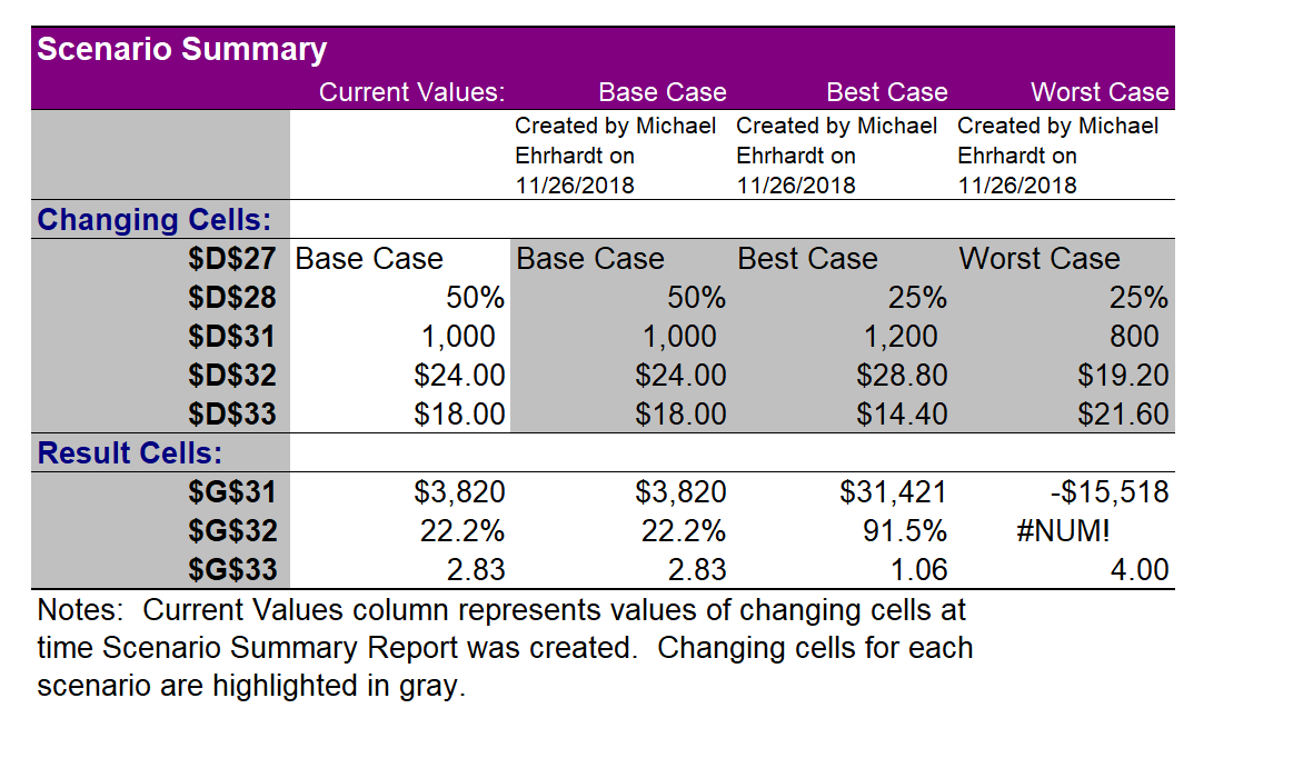

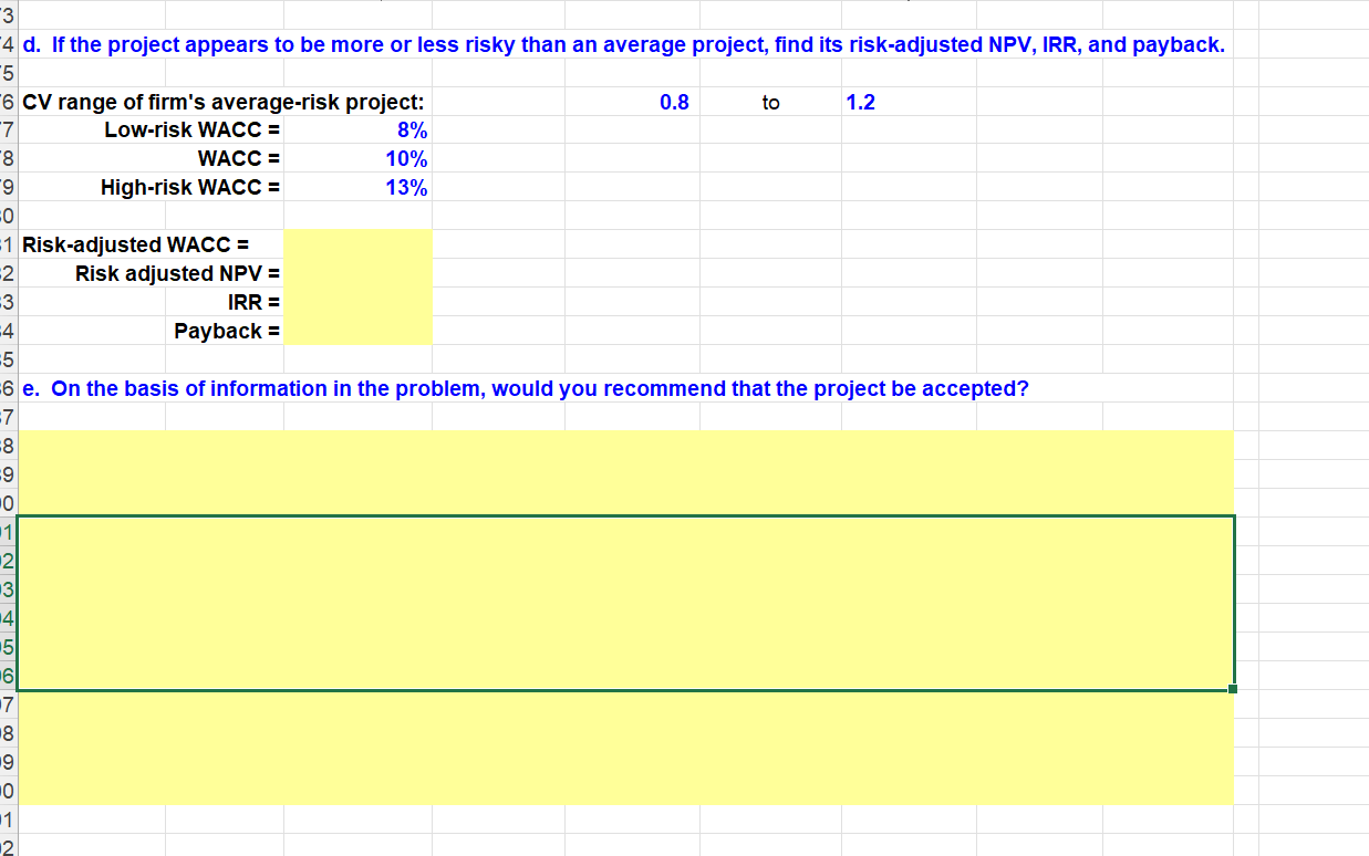
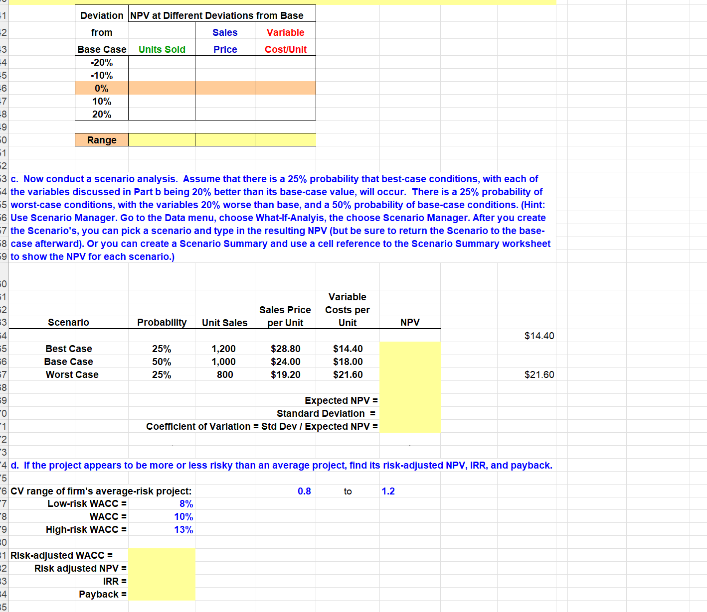
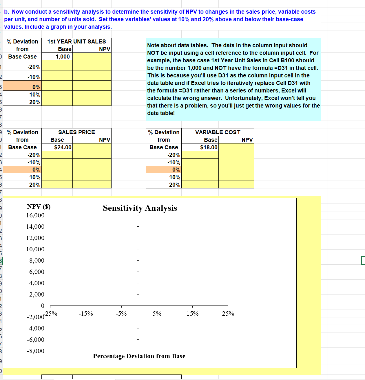
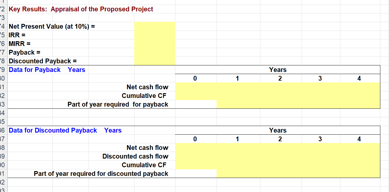
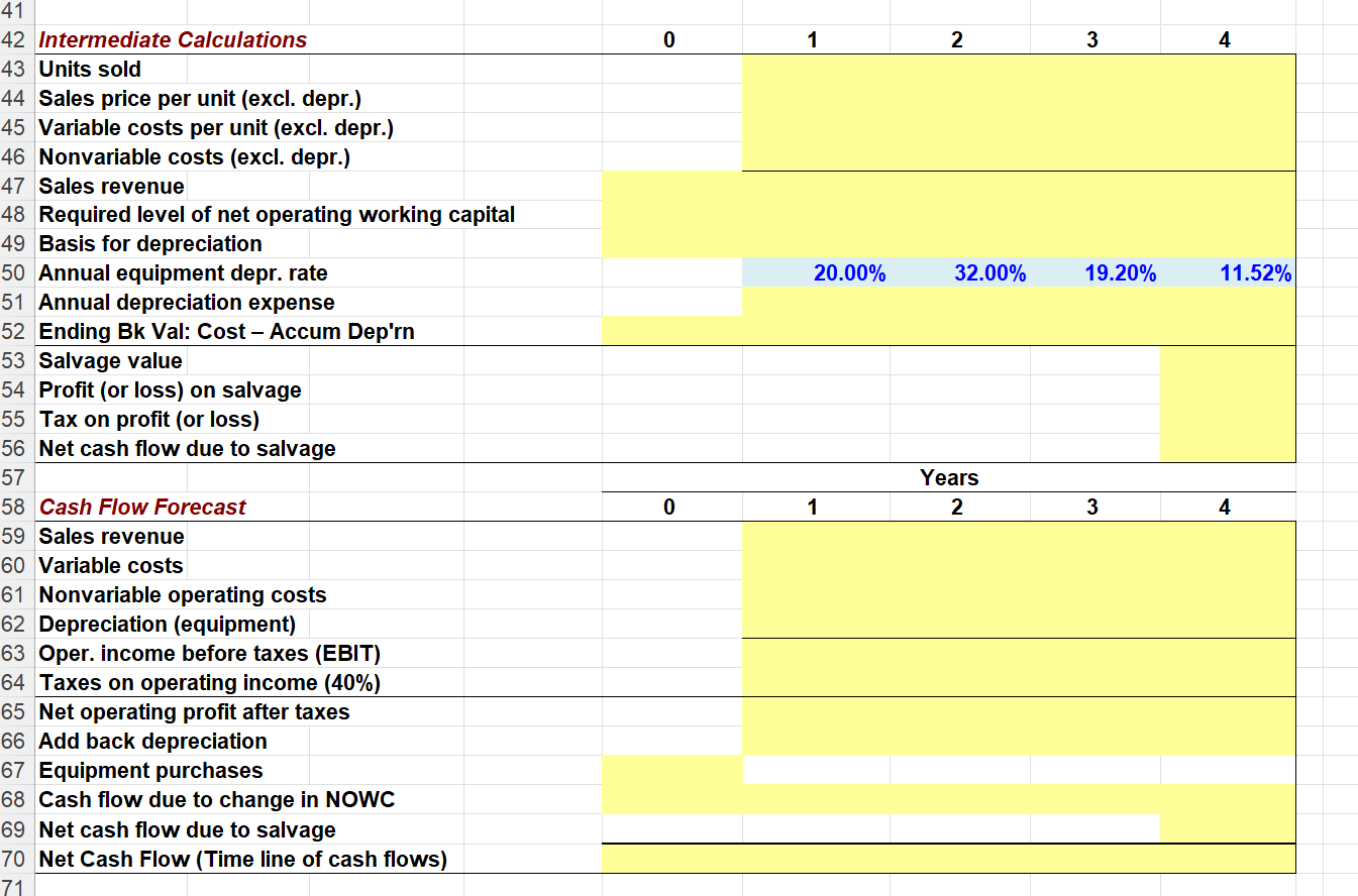
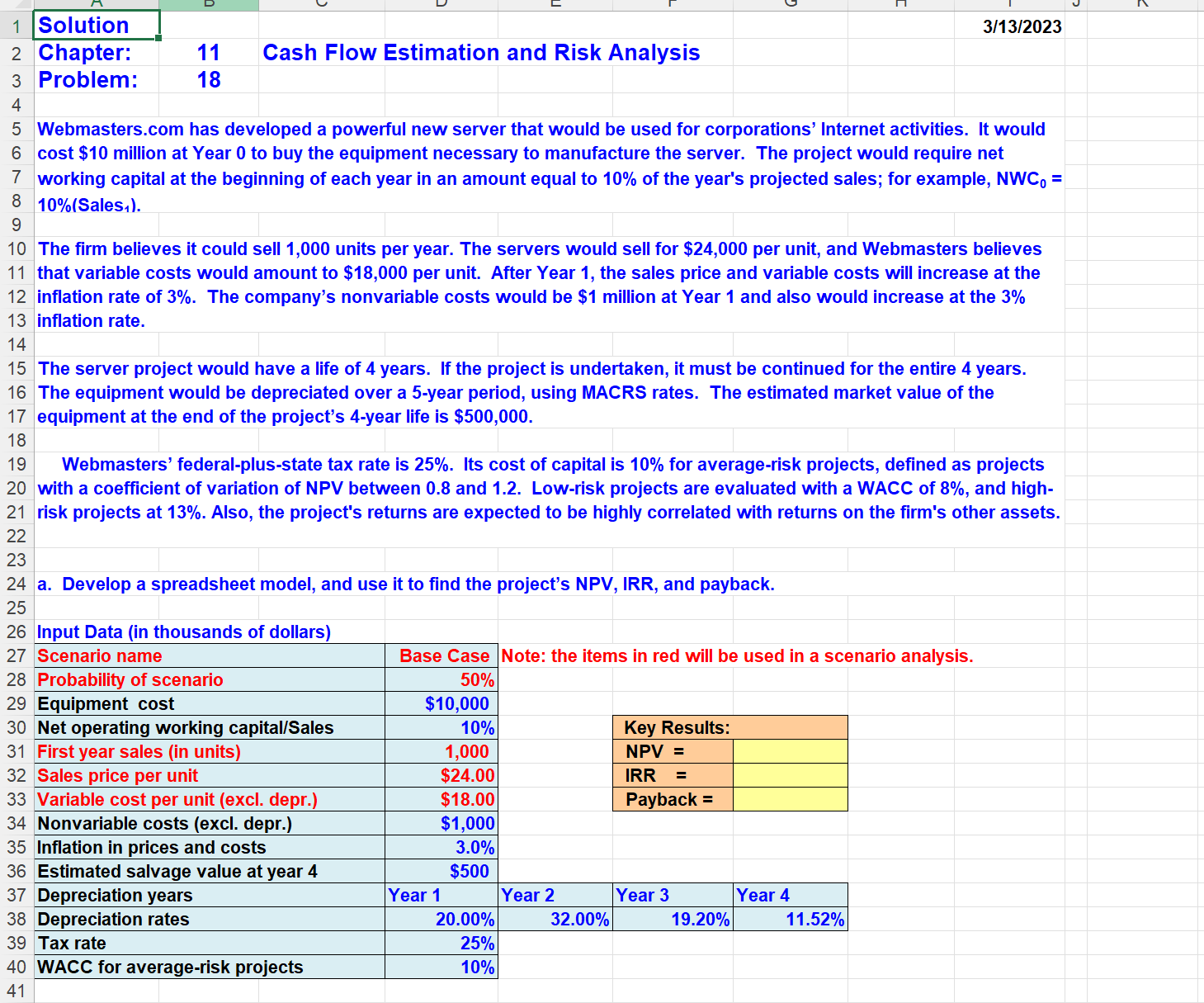
Notes: Current Values column represents values of changing cells at time Scenario Summary Report was created. Changing cells for each scenario are highlighted in gray. 3 4 d. If the project appears to be more or less risky than an average project, find its risk-adjusted NPV, IRR, and payback. 6 e. On the basis of information in the problem, would you recommend that the project be accepted? Key Results: Appraisal of the Proposed Project Net Present Value (at 10\%) = IRR = MIRR = Payback = Discounted Payback = Data for Payback Years Net cash flow Cumulative CF Part of year required for payback Data for Discounted Payback Years Net cash flow Discounted cash flow Cumulative CF Part of year required for discounted payback c. Now conduct a scenario analysis. Assume that there is a 25% probability that best-case conditions, with each of the variables discussed in Part b being 20% better than its base-case value, will occur. There is a 25% probability of worst-case conditions, with the variables 20% worse than base, and a 50% probability of base-case conditions. (Hint: Use Scenario Manager. Go to the Data menu, choose What-If-Analyis, the choose Scenario Manager. After you create the Scenario's, you can pick a scenario and type in the resulting NPV (but be sure to return the Scenario to the base-case afterward). Or you can create a Scenario Summary and use a cell reference to the Scenario Summary worksheet to show the NPV for each scenario.) 4 d. If the project appears to be more or less risky than an average project, find its risk-adjusted NPV, IRR, and payback. CV range of firm's average-risk project: Variable Sales Price Costs per Scenario Probability Unit Sales per Unit Unit NPV Best Case Base Case Worst Case 25% 50% 25% 1,200 1,000 800 $28.80 $24.00 $19.20 $14.40 $18.00 $21.60 $14.40 Expected NPV = Standard Deviation = Coefficient of Variation = Std Dev / Expected NPV = Low-risk WACC = WACC = High-risk WACC = 8% 10% 13% Risk-adjusted WACC = Risk adjusted NPV = IRR = Payback = 0.8 to 1.2 b. Now conduct a sensitivity analysis to determine the sensitivity of NPV to changes in the sales price, variable costs per unit, and number of units sold. Set these variables' values at 10% and 20% above and below their base-case values. Include a graph in your analysis. Note about data tables. The data in the column input should NOT be input using a cell reference to the column input cell. For example, the base case 1st Year Unit Sales in Cell B100 should be the number 1,000 and NOT have the formula =D31 in that cell. This is because you'll use D31 as the column input cell in the data table and if Excel tries to iteratively replace Cell D31 with the formula =D31 rather than a series of numbers, Excel will calculate the wrong answer. Unfortunately, Excel won't tell you that there is a problem, so you'll just get the wrong values for the data table! Notes: Current Values column represents values of changing cells at time Scenario Summary Report was created. Changing cells for each scenario are highlighted in gray. 3 4 d. If the project appears to be more or less risky than an average project, find its risk-adjusted NPV, IRR, and payback. 6 e. On the basis of information in the problem, would you recommend that the project be accepted? Key Results: Appraisal of the Proposed Project Net Present Value (at 10\%) = IRR = MIRR = Payback = Discounted Payback = Data for Payback Years Net cash flow Cumulative CF Part of year required for payback Data for Discounted Payback Years Net cash flow Discounted cash flow Cumulative CF Part of year required for discounted payback c. Now conduct a scenario analysis. Assume that there is a 25% probability that best-case conditions, with each of the variables discussed in Part b being 20% better than its base-case value, will occur. There is a 25% probability of worst-case conditions, with the variables 20% worse than base, and a 50% probability of base-case conditions. (Hint: Use Scenario Manager. Go to the Data menu, choose What-If-Analyis, the choose Scenario Manager. After you create the Scenario's, you can pick a scenario and type in the resulting NPV (but be sure to return the Scenario to the base-case afterward). Or you can create a Scenario Summary and use a cell reference to the Scenario Summary worksheet to show the NPV for each scenario.) 4 d. If the project appears to be more or less risky than an average project, find its risk-adjusted NPV, IRR, and payback. CV range of firm's average-risk project: Variable Sales Price Costs per Scenario Probability Unit Sales per Unit Unit NPV Best Case Base Case Worst Case 25% 50% 25% 1,200 1,000 800 $28.80 $24.00 $19.20 $14.40 $18.00 $21.60 $14.40 Expected NPV = Standard Deviation = Coefficient of Variation = Std Dev / Expected NPV = Low-risk WACC = WACC = High-risk WACC = 8% 10% 13% Risk-adjusted WACC = Risk adjusted NPV = IRR = Payback = 0.8 to 1.2 b. Now conduct a sensitivity analysis to determine the sensitivity of NPV to changes in the sales price, variable costs per unit, and number of units sold. Set these variables' values at 10% and 20% above and below their base-case values. Include a graph in your analysis. Note about data tables. The data in the column input should NOT be input using a cell reference to the column input cell. For example, the base case 1st Year Unit Sales in Cell B100 should be the number 1,000 and NOT have the formula =D31 in that cell. This is because you'll use D31 as the column input cell in the data table and if Excel tries to iteratively replace Cell D31 with the formula =D31 rather than a series of numbers, Excel will calculate the wrong answer. Unfortunately, Excel won't tell you that there is a problem, so you'll just get the wrong values for the data table