Please solve using Python
Please solve all questions The question asked is the misleading, and the one below it is the explanation of what is required
this is the picture


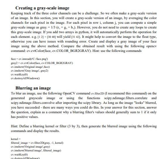
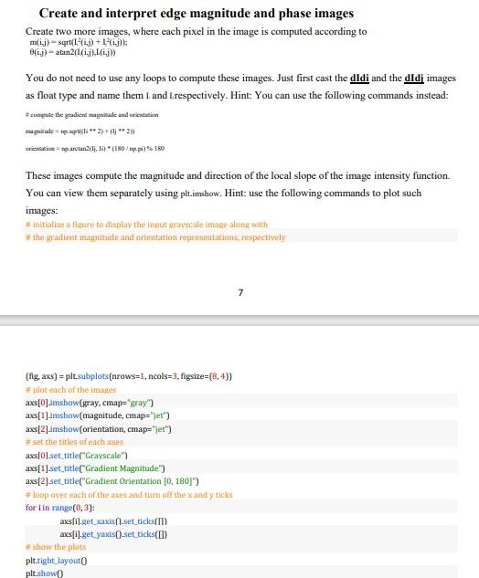
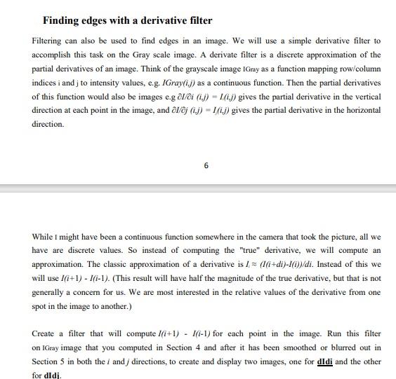
Creating a gray-scale image Keeping track of the three color channels can be a challenge. So we often make a gray-scale version of an image. In this section, you will create a gray-scale version of an image, by averaging the color channels for each pixel in the image. For each pixel in row i, column j, you can compute a simple gray-scale image as gray =1/3(r4+gj+b4). However, you do not need to create any loops to create this gray-scale image. If you add two arrays in python, it will automatically perform the operation for each element. e.g. [1 2]+[3040] will yield [31 42]. It might help to convert the image to the float type, otherwise you can have issues with rounding error. Create and display a gray image of your face image using the above method. Compare the obtained result with using the following opencv command: cv.cvtColor(face, cv.COLOR_BGR2GRAY). Hint: use the following commands face =cv.imread(r2C:/ face.pngh' gray2 = cv.cvtColor(face, cv_COLOR_BGR2GRAY) cv.imshow('Original image', face) cv.imshow('Gray image', gray2) cv. waitKey(0) cv.destroyAllWindows() Blurring an image To blur an image, use the following OpenCV command cv.filter2D (I recommend this command) on the generated grayscale image or using the functions scipy.ndimage.filters.correlate and scipy.ndimage.filters.convolve after importing the scipy library. As long as the image "looks" blurred, you have succeeded - there are many ways you could do this. In your answer for this section, answer the question, explain as a comment why a blurring filter's values should generally sum to 1 if it only has positive values. Hint: Define a blurring kernel or filter ( 3 by 3 ), then generate the blurred image using the following commands and display the results. ketnel = filtered image = cv.filter2D(gray, 1, kemel) cv.imshow('Original image', gray) cv.imshow('blurred image', filtered_inage) cv. waitKey (0) Create and interpret edge magnitude and phase images Create two more images, where each pixel in the image is computed according to m(i,j)=sqrt(L2(i,j)+12(i,j)), (i,j)=atan2(L(i,j),L(i,j)) You do not need to use any loops to compute these images. Just first cast the dIdi and the dIdi images as float type and name them 1 and l,respectively. Hint: You can use the following commands instead: * cumpute the gradient magrioude and orictatation magnitule = tp.sqpi(Ii 2)+(jj2)1 These images compute the magnitude and direction of the local slope of the image intensity function. You can view them separately using plt.imshow. Hint: use the following commands to plot such images: #t the gradient magnitude and orientation representations, respectively 7 (fig, axs) = plt.subplots[arows =1, ncols =3, figsize =(8,4) ) H plot each of the images axs[0]_imshow(gray, cmap= "gray") axs[1] limshow(magnitude, cmap="jet") axs[2] imshow(orientation, cmap= 'jet') if set the titlits of each axes axs[0]_set_title[ Crayscale"] axs[1]set_title["Gradient Magnitude") axs [2]set_title("Gradient Orientation [0, 180]7) # loop over each of the axes and turn off the x and y ticks for i in range (0,3) : axs[i].get_xaxis-set_ticksil] axs[i].get_yaxis[].set_ticks([]) * thenw the plats plt_tight,layout 0 plt.show0 Finding edges with a derivative filter Filtering can also be used to find edges in an image. We will use a simple derivative filter to accomplish this task on the Gray scale image. A derivate filter is a discrete approximation of the partial derivatives of an image. Think of the grayscale image IGray as a function mapping row/column indices i and j to intensity values, e.g. IGray (i,j) as a continuous function. Then the partial derivatives of this function would also be images e.g I/i(i,j)=Ii(ijj) gives the partial derivative in the vertical direction at each point in the image, and I/j(i,j)=I(i,j) gives the partial derivative in the horizontal direction. 6 While I might have been a continuous function somewhere in the camera that took the picture, all we have are discrete values. So instead of computing the "true" derivative, we will compute an approximation. The classic approximation of a derivative is Ii(I(i+di)I(i))/di. Instead of this we will use I(i+1)I(i1). (This result will have half the magnitude of the true derivative, but that is not generally a concern for us. We are most interested in the relative values of the derivative from one spot in the image to another.) Create a filter that will compute I(i+1)I(i1) for each point in the image. Run this filter on IGray image that you computed in Section 4 and after it has been smoothed or blurred out in Section 5 in both the i and j directions, to create and display two images, one for dldi and the other for dIdi. Creating a gray-scale image Keeping track of the three color channels can be a challenge. So we often make a gray-scale version of an image. In this section, you will create a gray-scale version of an image, by averaging the color channels for each pixel in the image. For each pixel in row i, column j, you can compute a simple gray-scale image as gray =1/3(r4+gj+b4). However, you do not need to create any loops to create this gray-scale image. If you add two arrays in python, it will automatically perform the operation for each element. e.g. [1 2]+[3040] will yield [31 42]. It might help to convert the image to the float type, otherwise you can have issues with rounding error. Create and display a gray image of your face image using the above method. Compare the obtained result with using the following opencv command: cv.cvtColor(face, cv.COLOR_BGR2GRAY). Hint: use the following commands face =cv.imread(r2C:/ face.pngh' gray2 = cv.cvtColor(face, cv_COLOR_BGR2GRAY) cv.imshow('Original image', face) cv.imshow('Gray image', gray2) cv. waitKey(0) cv.destroyAllWindows() Blurring an image To blur an image, use the following OpenCV command cv.filter2D (I recommend this command) on the generated grayscale image or using the functions scipy.ndimage.filters.correlate and scipy.ndimage.filters.convolve after importing the scipy library. As long as the image "looks" blurred, you have succeeded - there are many ways you could do this. In your answer for this section, answer the question, explain as a comment why a blurring filter's values should generally sum to 1 if it only has positive values. Hint: Define a blurring kernel or filter ( 3 by 3 ), then generate the blurred image using the following commands and display the results. ketnel = filtered image = cv.filter2D(gray, 1, kemel) cv.imshow('Original image', gray) cv.imshow('blurred image', filtered_inage) cv. waitKey (0) Create and interpret edge magnitude and phase images Create two more images, where each pixel in the image is computed according to m(i,j)=sqrt(L2(i,j)+12(i,j)), (i,j)=atan2(L(i,j),L(i,j)) You do not need to use any loops to compute these images. Just first cast the dIdi and the dIdi images as float type and name them 1 and l,respectively. Hint: You can use the following commands instead: * cumpute the gradient magrioude and orictatation magnitule = tp.sqpi(Ii 2)+(jj2)1 These images compute the magnitude and direction of the local slope of the image intensity function. You can view them separately using plt.imshow. Hint: use the following commands to plot such images: #t the gradient magnitude and orientation representations, respectively 7 (fig, axs) = plt.subplots[arows =1, ncols =3, figsize =(8,4) ) H plot each of the images axs[0]_imshow(gray, cmap= "gray") axs[1] limshow(magnitude, cmap="jet") axs[2] imshow(orientation, cmap= 'jet') if set the titlits of each axes axs[0]_set_title[ Crayscale"] axs[1]set_title["Gradient Magnitude") axs [2]set_title("Gradient Orientation [0, 180]7) # loop over each of the axes and turn off the x and y ticks for i in range (0,3) : axs[i].get_xaxis-set_ticksil] axs[i].get_yaxis[].set_ticks([]) * thenw the plats plt_tight,layout 0 plt.show0 Finding edges with a derivative filter Filtering can also be used to find edges in an image. We will use a simple derivative filter to accomplish this task on the Gray scale image. A derivate filter is a discrete approximation of the partial derivatives of an image. Think of the grayscale image IGray as a function mapping row/column indices i and j to intensity values, e.g. IGray (i,j) as a continuous function. Then the partial derivatives of this function would also be images e.g I/i(i,j)=Ii(ijj) gives the partial derivative in the vertical direction at each point in the image, and I/j(i,j)=I(i,j) gives the partial derivative in the horizontal direction. 6 While I might have been a continuous function somewhere in the camera that took the picture, all we have are discrete values. So instead of computing the "true" derivative, we will compute an approximation. The classic approximation of a derivative is Ii(I(i+di)I(i))/di. Instead of this we will use I(i+1)I(i1). (This result will have half the magnitude of the true derivative, but that is not generally a concern for us. We are most interested in the relative values of the derivative from one spot in the image to another.) Create a filter that will compute I(i+1)I(i1) for each point in the image. Run this filter on IGray image that you computed in Section 4 and after it has been smoothed or blurred out in Section 5 in both the i and j directions, to create and display two images, one for dldi and the other for dIdi

