please use Matlab to code this question.

equations 3.5-1 thru 3.5-7 are provided in the txt

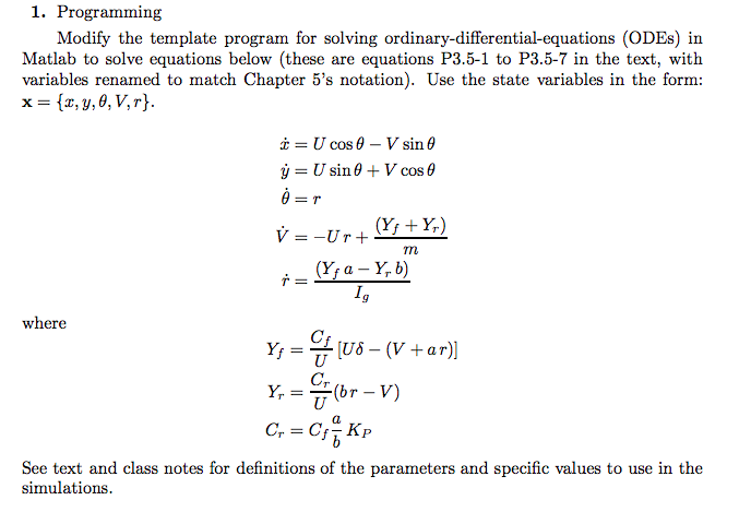
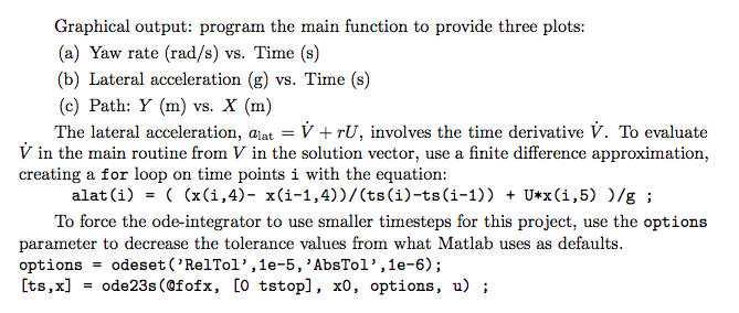
1. Programming Modify the template program for solving ordinary-differential-equations (ODEs) in Matlab to solve equations below (these are equations P3.5-1 to P3.5-7 in the text, with variables renamed to match Chapter 5's notation). Use the state variables in the form: x= {r, y, 6,V,r}. =U cos 6 - V sin y=U sin 0 + V cose 0=r m V = -Ur+ (Y; + Y) (Y;a - Y,6) = I. where Y; = (US - (v + ar) Y = Coy (or - V) Cr = Cs KP See text and class notes for definitions of the parameters and specific values to use in the simulations. Graphical output: program the main function to provide three plots: (a) Yaw rate (rad/s) vs. Time (s) (b) Lateral acceleration (g) vs. Time (s) (c) Path: Y (m) vs. X (m) The lateral acceleration, Qiat = V +rU, involves the time derivative V. To evaluate V in the main routine from V in the solution vector, use a finite difference approximation, creating a for loop on time points i with the equation: alat(i) = ( (x(i,4)- x(i-1,4))/(ts(i)-ts(i-1)) + U*x(1,5))/g ; To force the ode-integrator to use smaller timesteps for this project, use the options parameter to decrease the tolerance values from what Matlab uses as defaults. options odeset('RelTol', 1e-5, 'AbsTol', 12-6); [ts,x] = ode23s (@fofx, [O tstop], x0, options, u); 1. Programming Modify the template program for solving ordinary-differential-equations (ODEs) in Matlab to solve equations below (these are equations P3.5-1 to P3.5-7 in the text, with variables renamed to match Chapter 5's notation). Use the state variables in the form: x= {r, y, 6,V,r}. =U cos 6 - V sin y=U sin 0 + V cose 0=r m V = -Ur+ (Y; + Y) (Y;a - Y,6) = I. where Y; = (US - (v + ar) Y = Coy (or - V) Cr = Cs KP See text and class notes for definitions of the parameters and specific values to use in the simulations. Graphical output: program the main function to provide three plots: (a) Yaw rate (rad/s) vs. Time (s) (b) Lateral acceleration (g) vs. Time (s) (c) Path: Y (m) vs. X (m) The lateral acceleration, Qiat = V +rU, involves the time derivative V. To evaluate V in the main routine from V in the solution vector, use a finite difference approximation, creating a for loop on time points i with the equation: alat(i) = ( (x(i,4)- x(i-1,4))/(ts(i)-ts(i-1)) + U*x(1,5))/g ; To force the ode-integrator to use smaller timesteps for this project, use the options parameter to decrease the tolerance values from what Matlab uses as defaults. options odeset('RelTol', 1e-5, 'AbsTol', 12-6); [ts,x] = ode23s (@fofx, [O tstop], x0, options, u)