pls provide the full and correct answers

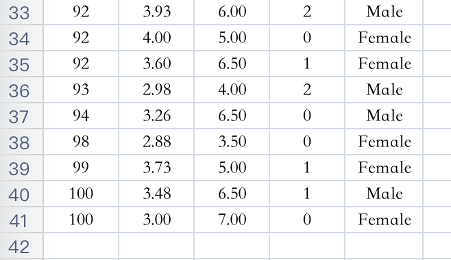
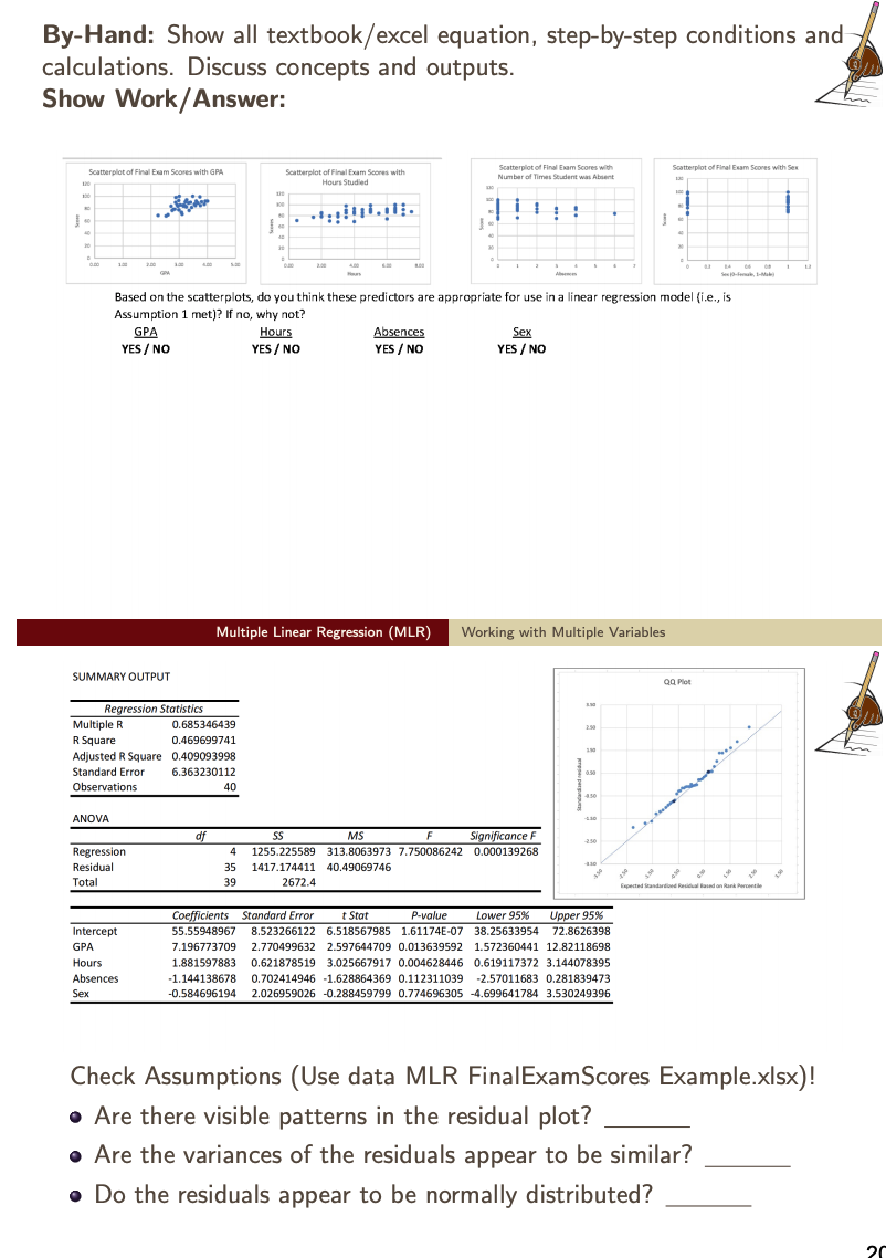
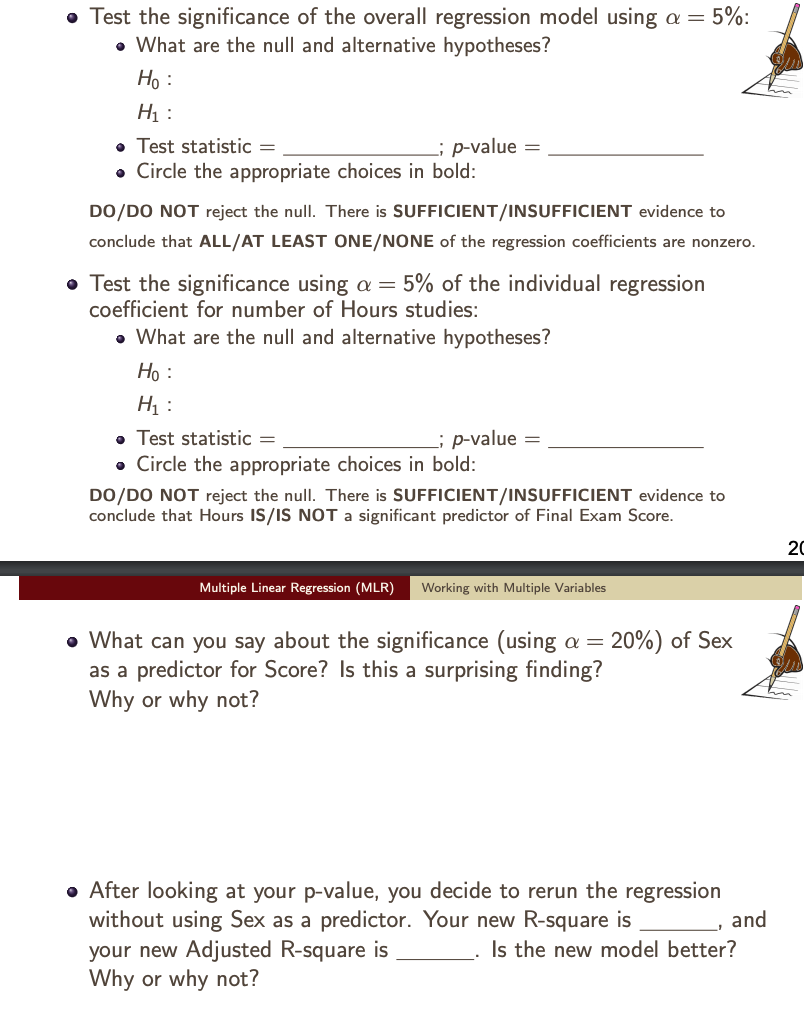
Score GPA Hours Absences Gender 2 68 2.53 3.00 0 Female 3 69 2.25 4.00 3 Female 4 70 2.60 2.50 Female 5 71 3.10 0.50 0 Male 6 74 3.08 6.00 4 Male 7 77 2.75 3.50 6 Female 8 77 3.35 1.50 0 Female 9 78 2.98 3.00 3 Male 10 78 2.99 2.00 3 Male 11 79 2.84 2.50 2 Male 12 79 2.80 4.50 0 Male 13 82 3.44 7.00 Female 14 83 3.25 3.00 Female 15 84 3.15 3.00 4 Female 16 84 3.18 5.50 0 Male 17 84 2.95 2.00 0 Female 18 84 2.71 4.00 Male 19 85 3.20 4.50 3 Female 20 85 3.75 2.00 0 Male 21 85 3.57 3.50 2 Female 22 86 2.92 6.00 Male 23 86 3.04 6.50 Female 24 86 3.16 5.00 3 Male 25 87 3.89 7.50 4 Female 26 87 3.54 4.00 0 Male 27 89 3.33 6.50 Male 28 89 3.66 5.00 O Male 29 90 2.87 3.50 Female 30 90 3.40 6.00 Female 31 91 3.22 4.50 N Female 32 91 3.79 7.00 0 Female 33 92 3.93 6.00 2 Male\fBy-Hand: Show all textbook/excel equation, step-by-step conditions and calculations. Discuss concepts and outputs. Show Work/ Answer: Scatterplot of Final Exam Scores with GPA Scatterplot of Final Exam Scores with Scatterplot of Final Exam Scores with Scatterplot of Final Exam Scores with Sex Hours Studied Number of Times Studer Based on the scatterplots, do you think these predictors are appropriate for use in a linear regression model (i.e., is Assumption 1 met)? If no, why not? GPA Hours Absences Sex YES / NO YES / NO YES / NO YES / NO Multiple Linear Regression (MLR) Working with Multiple Variables SUMMARY OUTPUT QQ Plot Regression Statistics Multiple R 0.685346439 2:50 Square 0.469699741 Adjusted R Square 0.409093998 Standard Error 6.363230112 Observations 40 450 ANOVA of SS MS Significance F 250 Regression 4 1255.225589 313.8063973 7.750086242 0.000139268 Residual 35 1417.174411 40.49069746 Total 39 2672.4 end Bound on funk Percent as Coefficients Standard Error t Stat P-value Lower 95% Upper 95% Intercept $5.55948967 8.523266122 6.518567985 1.61174E-07 38.25633954 72.8626398 GPA 7.196773709 2.770499632 2.597644709 0.013639592 1.572360441 12.82118698 Hours 1.881597883 0.621878519 3.025667917 0.004628446 0.619117372 3.144078395 Absences -1.144138678 0.702414946 -1.628864369 0.112311039 -2.57011683 0.281839473 Sex -0.584696194 2.026959026 -0.288459799 0.774696305 -4.699641784 3.530249396 Check Assumptions (Use data MLR FinalExamScores Example.xIsx)! . Are there visible patterns in the residual plot? . Are the variances of the residuals appear to be similar? . Do the residuals appear to be normally distributed?. Test the significance of the overall regression model using a = 5%: . What are the null and alternative hypotheses? Ho : H1 : . Test statistic = ; p-value = . Circle the appropriate choices in bold: DO/DO NOT reject the null. There is SUFFICIENT/INSUFFICIENT evidence to conclude that ALL/AT LEAST ONE/NONE of the regression coefficients are nonzero. . Test the significance using a = 5% of the individual regression coefficient for number of Hours studies: . What are the null and alternative hypotheses? Ho : H1 : . Test statistic = ; p-value = . Circle the appropriate choices in bold: DO/DO NOT reject the null. There is SUFFICIENT/INSUFFICIENT evidence to conclude that Hours IS/IS NOT a significant predictor of Final Exam Score. 2 Multiple Linear Regression (MLR) Working with Multiple Variables . What can you say about the significance (using a = 20%) of Sex as a predictor for Score? Is this a surprising finding? Why or why not? . After looking at your p-value, you decide to rerun the regression without using Sex as a predictor. Your new R-square is , and your new Adjusted R-square is . Is the new model better? Why or why not