portfolio performanxe and evaluation

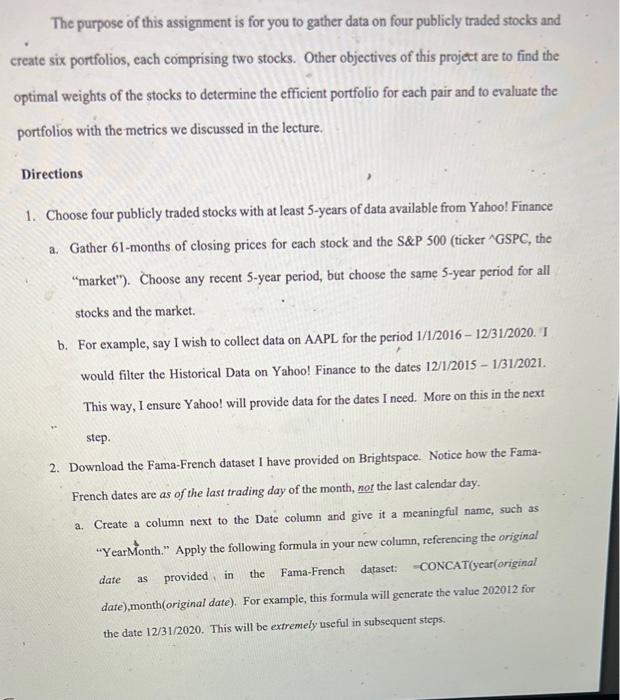
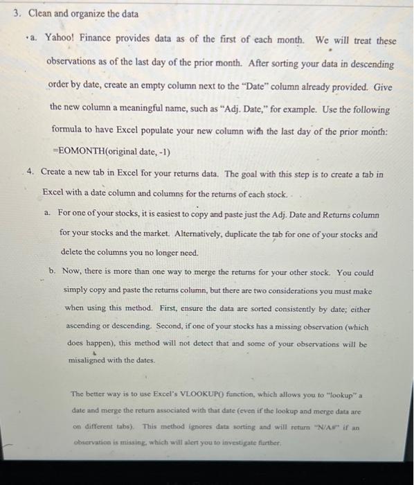
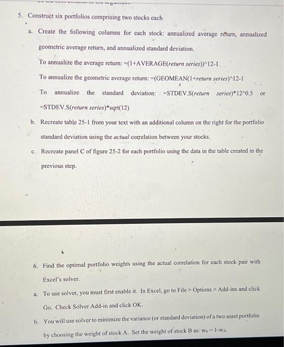
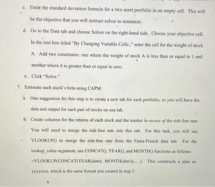
The purpose of this assignment is for you to gather data on four publicly traded stocks and create six portfolios, cach comprising two stocks. Other objectives of this project are to find the optimal weights of the stocks to determine the efficient portfolio for each pair and to evaluate the portfolios with the metrics we discussed in the lecture. Directions 1. Choose four publicly traded stocks with at least 5-years of data available from Yahoo! Finance a. Gather 61-months of closing prices for each stock and the S&P 500 (ticker GSPC, the "market"). Choose any recent 5-year period, but choose the same 5-year period for all stocks and the market. b. For example, say I wish to collect data on AAPL for the period 1/1/2016 - 12/31/2020. I would filter the Historical Data on Yahoo! Finance to the dates 12/1/2015 - 1/31/2021. This way, I ensure Yahoo! will provide data for the dates I need. More on this in the next step. 2. Download the Fama-French dataset I have provided on Brightspace. Notice how the Fama- French dates are as of the last trading day of the month, nor the last calendar day. a. Create a column next to the Date column and give it a meaningful name, such as "Year Month." Apply the following formula in your new column, referencing the original date provided in the Fama-French dataset: CONCAT(year(original date),month(original date). For example, this formula will generate the value 202012 for the date 12/31/2020. This will be extremely useful in subsequent steps. as 3. Clean and organize the data a. Yahoo! Finance provides data as of the first of each month. We will treat these observations as of the last day of the prior month. After sorting your data in descending order by date, create an empty column next to the Date" column already provided. Give the new column a meaningful name, such as Adj. Date," for example. Use the following formula to have Excel populate your new column with the last day of the prior month: =EOMONTH(original date, -1) 4. Create a new tab in Excel for your returns data. The goal with this step is to create a tab in Excel with a date column and columns for the returns of each stock. a. For one of your stocks, it is easiest to copy and paste just the Adj. Date and Returns column for your stocks and the market. Alternatively, duplicate the tab for one of your stocks and delete the columns you no longer need. b. Now, there is more than one way to merge the returns for your other stock. You could simply copy and paste the returns column, but there are two considerations you must make when using this method. First, ensure the data are sorted consistently by date; either ascending or descending. Second, if one of your stocks has a missing observation (which does happen), this method will not detect that and some of your observations will be misaligned with the dates. The better way is to use Excel's VLOOKUP() function, which allows you to "ookup" a date and merge the return associated with that date (even if the lookup and merge data are on different tabs). This method ignores data sorting and will return "N/Arif an observation is missing, which will alert you to investigate further 5. Construct six portfolios comprising two stocks each a. Create the following columns for cach stock: annualized average return, annualized geometric average return, and annualized standard deviation To annualize the average return: -(1+AVERAGE(return series)/12-1 To annualize the geometric average return: =(GEOMEAN(1+ return series) 12-1 To annualize the standard deviation: =STDEV.S(return series)* 12 0.5 or =STDEV.S(return series)*sqrt(12) b. Recreate table 25-1 from your text with an additional column on the right for the portfolio standard deviation using the actual corelation between your stocks. c. Recreate panel C of figure 25-2 for each portfolio using the data in the table created in the previous step. 6. Find the optimal portfolio weights using the actual correlation for each stock pair with Excel's solver a. To use solver, you must first enable it. In Excel, go to File > Options > Add-ins and click Go. Check Solver Add-in and click OK. b. You will use solver to minimize the variance (or standard deviation) of a two assct portfolio by choosing the weight of stock A. Set the weight of stock B as: Wb = 1-WA c. Enter the standard deviation formula for a two asset portfolio in an empty cell. This will be the objective that you will instruct solver to minimize. d. Go to the Data tab and choose Solver on the right-hand side. Choose your objective cell. In the text box titled "By Changing Variable Cells:," enter the cell for the weight of stock A. Add two constraints: one where the weight of stock A is less than or equal to 1 and another where it is greater than or equal to zero. e. Click "Solve." 7. Estimate each stock's beta using CAPM a. One suggestion for this step is to create a new tab for each portfolio, so you will have the data and output for each pair of stocks on one tab. b. Create columns for the returns of each stock and the market in excess of the risk-free rate. You will need to merge the risk-free rate into this tab. For this task, you will use VLOOKUPO to merge the risk-free rate from the Fama French data tab. For the lookup_value argument, use CONCATO, YEARO, and MONTH() functions as follows: =VLOOKUP(CONCAT(YEAR(date), MONTH(date))....). This constructs a date as yyyymm, which is the same format you created in step 2. c. Enable Excel's regression function by enabling the Analysis ToolPak following the same procedure as in step 6a. d. Excel's regression function is located on the Data menu > Data Analysis (far right of the menu). If you do not have Data Analysis as an option, go to File > Options > Add-ins, then click "Go..." at the bottom of the window next to Manage: Excel Add-ins. Check the box for Analysis ToolPak and click OK. e. Go to Data> Data Analysis > Regression. You must do this step individually for each stock. The excess stock returns are your "Input Y Range," and the excess market returns are your Input X Range. If you select the column labels, make sure to check the Labels" box on the regression window so Excel will ignore the first row of data (you'll get an error otherwise). Select the radio button next to Output Range and select an empty cell on the same tab for your regression output. Follow the same steps for the second stock in the portfolio, choosing an appropriate cell below or next to the regression output from the first stock. 8. Compute for each portfolio Jensen's alpha, Sharpe ratio, and Treynor ratio a. Calculate any additional risk or return metrics you deem necessary. 9. Write a report evaluating the performance of all six portfolios. Identify your winning portfolio and discuss what led you to that conclusion. There is no word count requirement for the written component, but it should be long enough to accommodate a cohesive and thorough discussion. Be sure to interpret your findings in steps 7 and 8. The purpose of this assignment is for you to gather data on four publicly traded stocks and create six portfolios, cach comprising two stocks. Other objectives of this project are to find the optimal weights of the stocks to determine the efficient portfolio for each pair and to evaluate the portfolios with the metrics we discussed in the lecture. Directions 1. Choose four publicly traded stocks with at least 5-years of data available from Yahoo! Finance a. Gather 61-months of closing prices for each stock and the S&P 500 (ticker GSPC, the "market"). Choose any recent 5-year period, but choose the same 5-year period for all stocks and the market. b. For example, say I wish to collect data on AAPL for the period 1/1/2016 - 12/31/2020. I would filter the Historical Data on Yahoo! Finance to the dates 12/1/2015 - 1/31/2021. This way, I ensure Yahoo! will provide data for the dates I need. More on this in the next step. 2. Download the Fama-French dataset I have provided on Brightspace. Notice how the Fama- French dates are as of the last trading day of the month, nor the last calendar day. a. Create a column next to the Date column and give it a meaningful name, such as "Year Month." Apply the following formula in your new column, referencing the original date provided in the Fama-French dataset: CONCAT(year(original date),month(original date). For example, this formula will generate the value 202012 for the date 12/31/2020. This will be extremely useful in subsequent steps. as 3. Clean and organize the data a. Yahoo! Finance provides data as of the first of each month. We will treat these observations as of the last day of the prior month. After sorting your data in descending order by date, create an empty column next to the Date" column already provided. Give the new column a meaningful name, such as Adj. Date," for example. Use the following formula to have Excel populate your new column with the last day of the prior month: =EOMONTH(original date, -1) 4. Create a new tab in Excel for your returns data. The goal with this step is to create a tab in Excel with a date column and columns for the returns of each stock. a. For one of your stocks, it is easiest to copy and paste just the Adj. Date and Returns column for your stocks and the market. Alternatively, duplicate the tab for one of your stocks and delete the columns you no longer need. b. Now, there is more than one way to merge the returns for your other stock. You could simply copy and paste the returns column, but there are two considerations you must make when using this method. First, ensure the data are sorted consistently by date; either ascending or descending. Second, if one of your stocks has a missing observation (which does happen), this method will not detect that and some of your observations will be misaligned with the dates. The better way is to use Excel's VLOOKUP() function, which allows you to "ookup" a date and merge the return associated with that date (even if the lookup and merge data are on different tabs). This method ignores data sorting and will return "N/Arif an observation is missing, which will alert you to investigate further 5. Construct six portfolios comprising two stocks each a. Create the following columns for cach stock: annualized average return, annualized geometric average return, and annualized standard deviation To annualize the average return: -(1+AVERAGE(return series)/12-1 To annualize the geometric average return: =(GEOMEAN(1+ return series) 12-1 To annualize the standard deviation: =STDEV.S(return series)* 12 0.5 or =STDEV.S(return series)*sqrt(12) b. Recreate table 25-1 from your text with an additional column on the right for the portfolio standard deviation using the actual corelation between your stocks. c. Recreate panel C of figure 25-2 for each portfolio using the data in the table created in the previous step. 6. Find the optimal portfolio weights using the actual correlation for each stock pair with Excel's solver a. To use solver, you must first enable it. In Excel, go to File > Options > Add-ins and click Go. Check Solver Add-in and click OK. b. You will use solver to minimize the variance (or standard deviation) of a two assct portfolio by choosing the weight of stock A. Set the weight of stock B as: Wb = 1-WA c. Enter the standard deviation formula for a two asset portfolio in an empty cell. This will be the objective that you will instruct solver to minimize. d. Go to the Data tab and choose Solver on the right-hand side. Choose your objective cell. In the text box titled "By Changing Variable Cells:," enter the cell for the weight of stock A. Add two constraints: one where the weight of stock A is less than or equal to 1 and another where it is greater than or equal to zero. e. Click "Solve." 7. Estimate each stock's beta using CAPM a. One suggestion for this step is to create a new tab for each portfolio, so you will have the data and output for each pair of stocks on one tab. b. Create columns for the returns of each stock and the market in excess of the risk-free rate. You will need to merge the risk-free rate into this tab. For this task, you will use VLOOKUPO to merge the risk-free rate from the Fama French data tab. For the lookup_value argument, use CONCATO, YEARO, and MONTH() functions as follows: =VLOOKUP(CONCAT(YEAR(date), MONTH(date))....). This constructs a date as yyyymm, which is the same format you created in step 2. c. Enable Excel's regression function by enabling the Analysis ToolPak following the same procedure as in step 6a. d. Excel's regression function is located on the Data menu > Data Analysis (far right of the menu). If you do not have Data Analysis as an option, go to File > Options > Add-ins, then click "Go..." at the bottom of the window next to Manage: Excel Add-ins. Check the box for Analysis ToolPak and click OK. e. Go to Data> Data Analysis > Regression. You must do this step individually for each stock. The excess stock returns are your "Input Y Range," and the excess market returns are your Input X Range. If you select the column labels, make sure to check the Labels" box on the regression window so Excel will ignore the first row of data (you'll get an error otherwise). Select the radio button next to Output Range and select an empty cell on the same tab for your regression output. Follow the same steps for the second stock in the portfolio, choosing an appropriate cell below or next to the regression output from the first stock. 8. Compute for each portfolio Jensen's alpha, Sharpe ratio, and Treynor ratio a. Calculate any additional risk or return metrics you deem necessary. 9. Write a report evaluating the performance of all six portfolios. Identify your winning portfolio and discuss what led you to that conclusion. There is no word count requirement for the written component, but it should be long enough to accommodate a cohesive and thorough discussion. Be sure to interpret your findings in steps 7 and 8