Predator-Prey Simulation
Population balance models are common ways to examine how interdependencies among entities dictate those entities' populations over time. A simple predator-prey population balance model might stipulate four important rates:
Prey animals reproduce and die naturally. In the absence of any predators, the rate at which the prey population increases due to births and deaths is proportional to the prey population (call this proportionality constant "'');
Prey animals are eaten by predators. The rate at which the prey population decreases due to predation is proportional to the product of the predator and prey populations (call this proportionality constant "");
Predators die off without prey. In the absence of any prey, the rate at which the predator population decreases due to births and deaths is proportional to the predator population (call this proportionality constant "");
Predators will reproduce faster if prey is available. The rate at which predatory population increases due to predation is proportional to the product of the predator and prey populations (call this proportionality constant "").
Credit: Kennedy News and Media
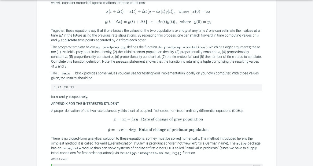
Let and be the population of prey and predators, respectively, per unit land area (that is, we mean these to be population densities so we can use calculus to model them). With the rates defined above, and a stipulation of the initial values of and , a rate-balance model allows one to predict and at any future time . A proper derivation of the rate balance equations is given in the Appendix below; for now, we will consider numerical approximations to those equations:
Together, these equations say that if one knows the values of the two populations and at any time one can estimate their values at a time in the future using the previous rate stipulations. By repeating this process, one can march forward in time computing values of and at discrete time points separated by from each other.
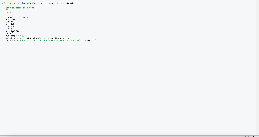
The program template below, my_predprey.py, defines the function do_predprey_simulation() which has eight arguments; these are (1) the initial prey population density, (2) the initial predator population density, (3) proportionality constant , (4) proportionality constant , (5) proportionality constant , (6) proportionality constant , (7) the time-step , and (8) the number of time steps to simulate. Complete this function definition. Note the return statement shows that the function is returning a tuple comprising the resulting values of x and y.
The __main__ block provides some values you can use for testing your implementation locally on your own computer. With those values given, the results should be
0.41 28.72
for x and y, respectively.
APPENDIX FOR THE INTERESTED STUDENT
A proper derivation of the two rate balances yields a set of coupled, first-order, non-linear, ordinary differential equations (ODEs):
There is no closed-form analytical solution to these equations, so they must be solved numerically. The method introduced here is the simplest method; it is called "forward Euler integration" ("Euler" is pronounced "oiler" not "yew-ler"; it's a German name). The scipy package has an integrate module than can solve systems of nonlinear first-order ODE's called "initial value problems" (since we have to supply initial conditions for first-order equations) via the scipy.integrate.solve_ivp() function.
5.27 Program Project 1: Predator-Prey Simulation Population balance models are common ways to examine how interdependencies among entities dictate those entities' populations over time. A simple predator-prey population balance model might stipulate four important rates: Prey animals reproduce and die naturally. In the absence of any predators, the rate at which the prey population increases due to births and deaths is proportional to the prey population (call this proportionality constant'a"); Prey animals are eaten by predators. The rate at which the prey population decreases due to predation is proportional to the product of the predator and prey populations (call this proportionality constant'"); Predators die off without prey. In the absence of any prey, the rate at which the predator population decreases due to births and deaths is proportional to the predator population (call this proportionality constante"); Predators will reproduce faster if prey is available. The rate at which predatory population increases due to predation is proportional to the product of the predator and prey populations (call this proportionality constantl"). Credit Kennecy News and Media Leta andy be the population of prey and predators, respectively, per unit land area (that is, we mean these to be population densities so we can use calculus to model them). With the rates defined above, and a stipulation of the initial values of sand y, a rate balance model allows one to predict . and y at any future time t. A proper derivation of the rate balance equations is given in the Appendix below, for now, we will consider numerical approximations to those equations: we will consider numerical approximations to those equations: 2(t+At) = x(t) + At a-bu(t)y(t), where (0) = 20 ylt + At) = y(t) + At[-c+de(t)y(t)], where y(0) = yo Together, these equations say that if one knows the values of the two populations and y at any time / one can estimate their values at a time At in the future using the previous rate stipulations. By repeating this process, one can march forward in time computing values of a and y at discrete time points separated by At from each other. The program template below, my_predprey.py, defines the function do_predprey_simulation () which has eight arguments; these are (1) the initial prey population density (2) the initial predator population density (3) proportionality constante, (4) proportionality constant, (5) proportionality constant (6) proportionality constant d. (7) the time-step At, and (a) the number of time steps to simulate Complete this function definition. Note the return statement shows that the function is returning a tuple comprising the resulting values of x and y The __main__block provides some values you can use for testing your implementation locally on your own computer. With those values given, the results should be 0.41 28.72 for x and y, respectively APPENDIX FOR THE INTERESTED STUDENT A proper derivation of the two rate balances yields a set of coupled, first-order, non-linear, ordinary differential equations (ODES) = 22 - bay Rate of change of prey population y=-cx+dry Rate of change of predator population There is no closed-form analytical solution to these equations, so they must be solved numerically. The method introduced here is the simplest method, it is called 'forward Euler integration' ("Euler' is pronounced oiler" not "yew-ler" it's a German name). The scipy package has an integrate module than can solve systems of nonlinear first-order ODEs called 'initial value problems' (since we have to supply initial conditions for first-order equations) via the scipy integrate.solve_ivp() function. 28018317255 der do_predprey_sinulation x, ya, b, a, d, dt, num_steps: Your solution goes here relumn (xiv if nane --' main': x - 1999 y = 22 a = 2.1 b.61 -3.91 d = 2.99889 dt = 4,3 nun staps = 150 x,y-do_pred_prey_sinulationix, y, a,b,c,d, at, nun_steps: print Prey density is (:.21), and predator density is 1:21)'.format(x,y) 5.27 Program Project 1: Predator-Prey Simulation Population balance models are common ways to examine how interdependencies among entities dictate those entities' populations over time. A simple predator-prey population balance model might stipulate four important rates: Prey animals reproduce and die naturally. In the absence of any predators, the rate at which the prey population increases due to births and deaths is proportional to the prey population (call this proportionality constant'a"); Prey animals are eaten by predators. The rate at which the prey population decreases due to predation is proportional to the product of the predator and prey populations (call this proportionality constant'"); Predators die off without prey. In the absence of any prey, the rate at which the predator population decreases due to births and deaths is proportional to the predator population (call this proportionality constante"); Predators will reproduce faster if prey is available. The rate at which predatory population increases due to predation is proportional to the product of the predator and prey populations (call this proportionality constantl"). Credit Kennecy News and Media Leta andy be the population of prey and predators, respectively, per unit land area (that is, we mean these to be population densities so we can use calculus to model them). With the rates defined above, and a stipulation of the initial values of sand y, a rate balance model allows one to predict . and y at any future time t. A proper derivation of the rate balance equations is given in the Appendix below, for now, we will consider numerical approximations to those equations: we will consider numerical approximations to those equations: 2(t+At) = x(t) + At a-bu(t)y(t), where (0) = 20 ylt + At) = y(t) + At[-c+de(t)y(t)], where y(0) = yo Together, these equations say that if one knows the values of the two populations and y at any time / one can estimate their values at a time At in the future using the previous rate stipulations. By repeating this process, one can march forward in time computing values of a and y at discrete time points separated by At from each other. The program template below, my_predprey.py, defines the function do_predprey_simulation () which has eight arguments; these are (1) the initial prey population density (2) the initial predator population density (3) proportionality constante, (4) proportionality constant, (5) proportionality constant (6) proportionality constant d. (7) the time-step At, and (a) the number of time steps to simulate Complete this function definition. Note the return statement shows that the function is returning a tuple comprising the resulting values of x and y The __main__block provides some values you can use for testing your implementation locally on your own computer. With those values given, the results should be 0.41 28.72 for x and y, respectively APPENDIX FOR THE INTERESTED STUDENT A proper derivation of the two rate balances yields a set of coupled, first-order, non-linear, ordinary differential equations (ODES) = 22 - bay Rate of change of prey population y=-cx+dry Rate of change of predator population There is no closed-form analytical solution to these equations, so they must be solved numerically. The method introduced here is the simplest method, it is called 'forward Euler integration' ("Euler' is pronounced oiler" not "yew-ler" it's a German name). The scipy package has an integrate module than can solve systems of nonlinear first-order ODEs called 'initial value problems' (since we have to supply initial conditions for first-order equations) via the scipy integrate.solve_ivp() function. 28018317255 der do_predprey_sinulation x, ya, b, a, d, dt, num_steps: Your solution goes here relumn (xiv if nane --' main': x - 1999 y = 22 a = 2.1 b.61 -3.91 d = 2.99889 dt = 4,3 nun staps = 150 x,y-do_pred_prey_sinulationix, y, a,b,c,d, at, nun_steps: print Prey density is (:.21), and predator density is 1:21)'.format(x,y)