Predicting Airfare on New Routes:

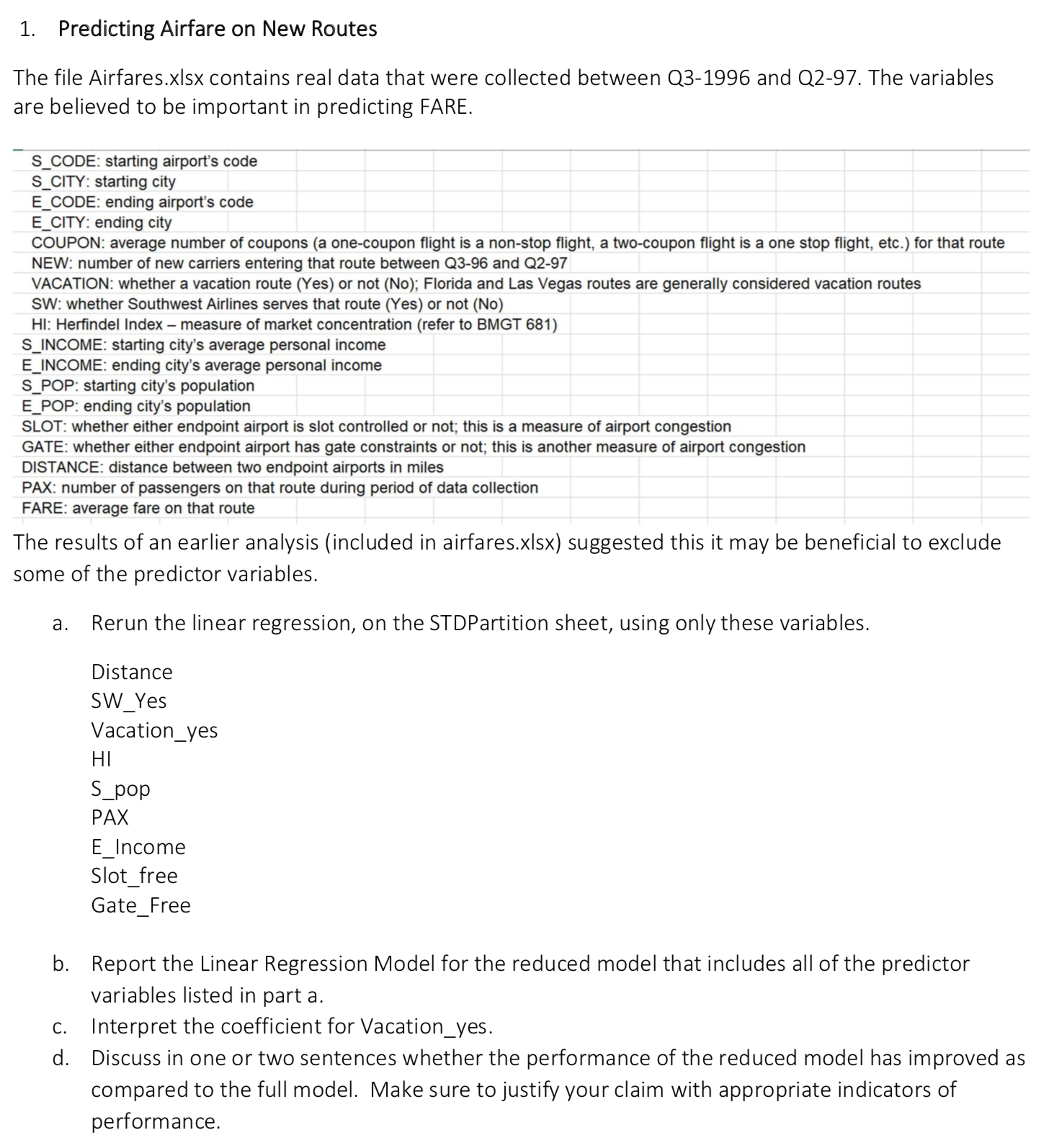
1. Predicting Airfare on New Routes The file Airfaresxlsx contains real data that were collected between 031996 and (1297. The variables are believed to be important in predicting FARE. S_CODE: starting airport's code S_CITY: starting city E_CODE: ending airport's code E_CITY: ending city COUPON: average number of coupons (a one-coupon ight is a non-stop ight. a two-coupon ight is a one stop ight, etc.) for that route NEW: number of new carriers entering that route between 03-96 and 02-97 VACATION: whether a vacation route (Yes) or not (No); Florida and Las Vegas routes are generally considered vacation routes SW: whether Southwest Airlines serves that route (Yes) or not (No) H1: Herndel Index measure at market concentration (refer to BMGT 681) S_INCOME: starting city's average personal income E_INCOME: ending city's average personal income S_POP: starting city's population E_POP: ending city's population SLOT: whether either endpoint airport is slot controlled or not; this is a measure of airport congestion GATE: whether either endpoint airport has gate constraints or not; this is another measure of airport congestion DISTANCE: distance between two endpoint airports in miles PAX: number of passengers on that route during period of data collection FARE: average fare on that route The results of an earlier analysis (included in airfaresxlsx) suggested this it may be beneficial to exclude some of the predictor variables. a. Rerun the linear regression, on the STDPartition sheet, using only these variables. Distance SW_Yes Vacation_yes HI S_pop PAX E_Income Slot_free Gate_Free b. Report the Linear Regression Model for the reduced model that includes all ofthe predictor variables listed in part a. c. Interpret the coefficient for Vacation_yes. d. Discuss in one or two sentences whether the performance of the reduced model has improved as compared to the full model. Make sure to justify your claim with appropriate indicators of performance