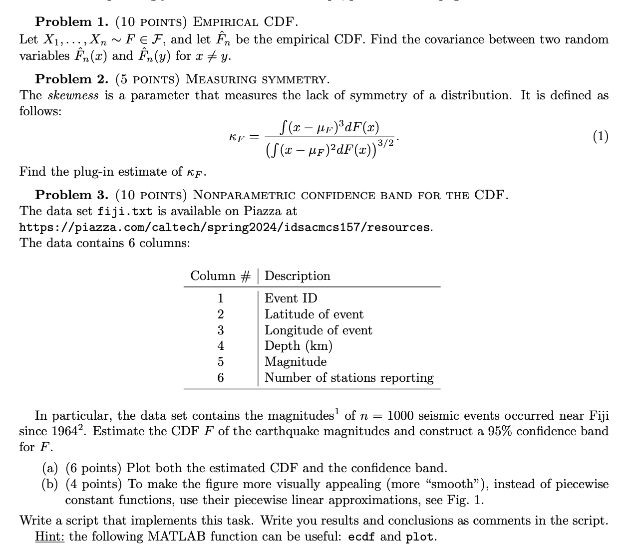
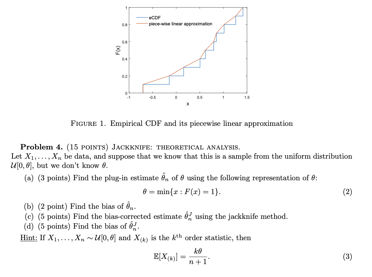
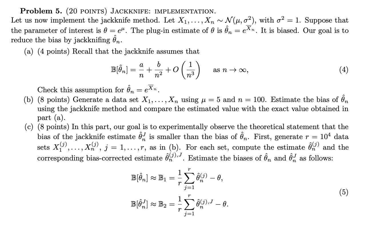
Problem 1. (10 POINTS) EMPIRICAL CDF. Let X1,..., Xn ~ F , and let be the empirical CDF. Find the covariance between two random variables Fn(x) and Fn(y) for x + y. Problem 2. (5 POINTS) MEASURING SYMMETRY. The skewness is a parameter that measures the lack of symmetry of a distribution. It is defined as follows: KF = (x F)dF(x) ((x F)dF(x)) /2 Find the plug-in estimate of KF. Problem 3. (10 POINTS) NONPARAMETRIC CONFIDENCE BAND FOR THE CDF. The data set fiji.txt is available on Piazza at https://piazza.com/caltech/spring2024/idsacmcs157/resources. The data contains 6 columns: Column # Description 1 2 Event ID Latitude of event Longitude of event Depth (km) 3 4 5 Magnitude 6 Number of stations reporting (1) In particular, the data set contains the magnitudes of n = 1000 seismic events occurred near Fiji since 1964. Estimate the CDF F of the earthquake magnitudes and construct a 95% confidence band for F. (a) (6 points) Plot both the estimated CDF and the confidence band. (b) (4 points) To make the figure more visually appealing (more "smooth"), instead of piecewise constant functions, use their piecewise linear approximations, see Fig. 1. Write a script that implements this task. Write you results and conclusions as comments in the script. Hint: the following MATLAB function can be useful: ecdf and plot. F(x) 1 0.8 eCDF piece-wise linear approximation 0.6 0.4 0.2 0 -1 -0.5 0 0.5 1 1.5 X FIGURE 1. Empirical CDF and its piecewise linear approximation Problem 4. (15 POINTS) JACKKNIFE: THEORETICAL ANALYSIS. Let X1,..., Xn be data, and suppose that we know that this is a sample from the uniform distribution U[0,0], but we don't know 0. (a) (3 points) Find the plug-in estimate n of 0 using the following representation of 0: (b) (2 point) Find the bias of n. = min{x : F(x) = 1}. (c) (5 points) Find the bias-corrected estimate 62 using the jackknife method. (d) (5 points) Find the bias of . Hint: If X, , Xn ~U[0,0] and X(k) is the kth order statistic, then (2) kO E[X(k)] = = n+1 (3) ~ N(, ), with o = 1. Suppose that Problem 5. (20 POINTS) JACKKNIFE: IMPLEMENTATION. Let us now implement the jackknife method. Let X,.. Xn the parameter of interest is 0 = e". The plug-in estimate of 0 is m = ex. It is biased. Our goal is to reduce the bias by jackknifing n. (a) (4 points) Recall that the jackknife assumes that a b + n n B[n] - Check this assumption for n = = exn +0 () as n, (4) (b) (8 points) Generate a data set X1, ..., X, using = 5 and n = 100. Estimate the bias of n using the jackknife method and compare the estimated value with the exact value obtained in part (a). (c) (8 points) In this part, our goal is to experimentally observe the theoretical statement that the bias of the jackknife estimate 6 is smaller than the bias of n. First, generate r = 104 data X(j), j = 1,...,r, as in (b). For each set, compute the estimate 6 (5) and the corresponding bias-corrected estimate A (1), J. Estimate the biases of n and as follows: sets (j), 90009 r 1 B[n] B1 B[0] B2 = IM - (j) 0, `(j), - - 0. (5) Compute both B1 and B2. We expect B to be approximately equal to the exact value given by (4), and to be larger (in absolute value) than B2. Write a script that implements the tasks in parts (b) and (c). Write you results and conclusions as comments in the script. = Hint: If X ~ N(, o), then Y particular, E[Y] = e"+02. Also the following MATLAB functions can be useful: randn and cat. e follows the log-normal distribution, Y ~ In N(, o). In