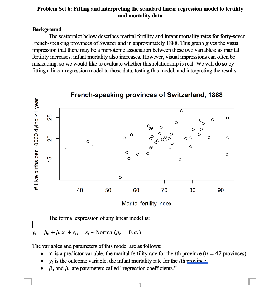
Problem Set 6: Fitting and interpreting the standard linear regression model to fertility and mortality data Background The scatterplot below describes marital fertility and infant mortality rates for forty-seven French-speaking provinces of Switzerland in approximately 1888. This graph gives the visual impression that there may be a monotonic association between these two variables: as marital fertility increases, infant mortality also increases. However, visual impressions can often be misleading, so we would like to evaluate whether this relationship is real. We will do so by tting a linear regression model to these data, testing this model, and interpreting the results. 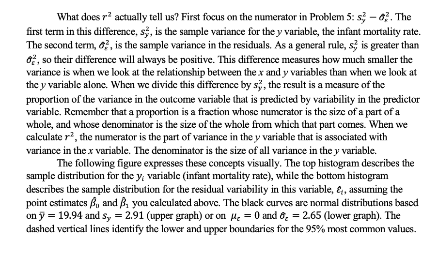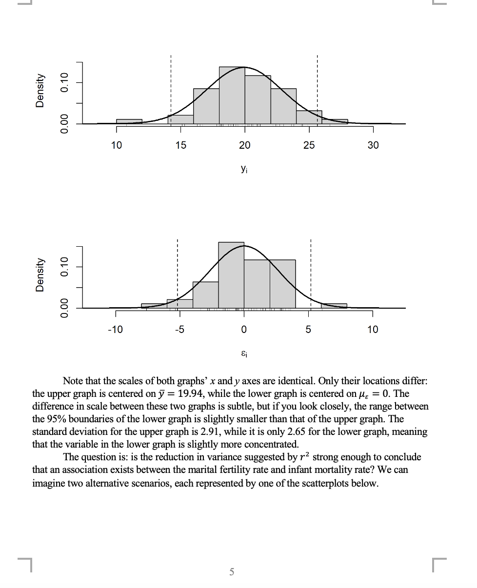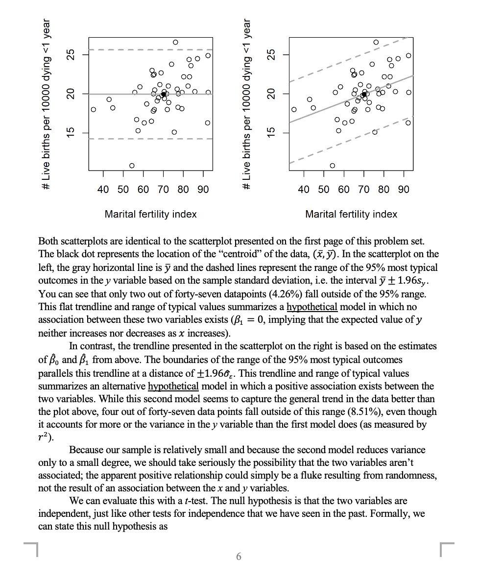French-speaking provinces of Switzerland, 1888 # Live births per 10000 dying 1 C.) .4: \\ 2 c: (1) D Q C! 0 >-. C) r': \\ 2 D (1) D 0.00 Note that the scales of both graphs' 3: and y axes are identical. Only their locations di'er: the upper graph is centered on 37 = 19.94, while the lower graph is centered on .115 = 0. The difference in scale between these two graphs is subtle, but ifyou look closely, the range between the 95% boundaries of the lower graph is slightly smaller than that of the upper graph. The standard deviation for the upper graph is 2.91, while it is only 2.65 for the lower graph, meaning that the variable in the lower graph is slightly more concentrated The question is: is the reduction in variance suggested by r2 strong enough to conclude that an association exists between the marital fertility rate and infant mortality rate? We can imagine two alternative scenarios, each represented by one of the scatterplots below. [ at to to an >~ an . 0 ' 0,! V '00 ------------ V LD 4" a: N 000 a: N ,' 000 t: 0 0 I: I, 0 O ._ ._ , 1:5\" %0 00 Pg" ,\" ($0 00 o o 00 o o 0 00 o c: c: C!_ o 8 00 8 N O o 0 8 N 0 ' 0 QOCO ' o 0 90% 3g 000 o g 000 ,z'o In to 0') \\ ____0____0____ to 1_ O \"U .: .t: ,r .E' E ,' .o .r: ,x a: a: -' .2 O .2 0 _l _l =11: at 40 50 60 70 80 90 40 50 60 70 80 90 Marital fertility index Marital fertility index Both scatterplots are identical to the scatterplot presented on the rst page of this problem set. The black dot represents the location of the \"centroi \" of the data, (1?. 37). In the scatterplot on the left, the gray horizontal line is y and the dashed lines represent the range of the 95% most typical outcomes in they variable based on the sample standard deviation, i.e. the interval 3? i 1.965),. You can see that only two out of forty-seven datapoints (4.26%) fall outside of the 95% range. This at trendline and range of typical values summarizes a hypgthetical model in which no association between these two variables exists (131 = 0, implying that the expected value of y neither increases nor decreases as 1: increases). In contrast, the trendline presented in the scatterplot on the right is based on the estimates of BB and 31 om above. The boundaries of the range of the 95% most typical outcomes parallels this trendline at a distance of $1.960}. This trendline and range of typical values summarizes an alternative hypgthetical model in which a positive association exists between the two variables. While this second model seems to capture the general trend in the data better than the plot above, four out of forty-seven data points fall outside of this range (8.51%), even though it accounts for more or the variance in they variable than the rst model does (as measured by F). Because our sample is relatively small and because the second model reduces variance only to a small degree, we should take seriously the possibility that the tw0 variables aren't associated; the apparent positive relationship could simply be a uke resulting om randomness, not the result of an association between the x and y variables. We can evaluate this with a ttest. The null hypothesis is that the two variables are independent, just like other tests for independence that we have seen in the past. Formally, we can state this null hypothesis as _| 6 Ho: Bi = 0 (Here, the asterisk is used to indicate that this is a hypothetical rather than known value.) The first step is to calculate a T test statistic that incorporates our point estimate ,, our hypothesized value of Bi, and the standard error for our point estimate. Calculating standard errors for regression coefficients is hard, so I will simply tell you that in this case, it is SE = 0.0316 (7) Tobs = B1 - Bi. SE Next, we need to determine the degrees of freedom (d. f.) for the t-distribution relevant for this test. For t-tests for regression coefficients, d. f. is equal to sample size minus the number of regression coefficients included in the model, in this case two (Bo and B,) (8) d.f. = Let us set our level of significance to a = 0.01. For this significance level and the degrees of freedom you calculated in Problem 8, what is the critical value for the T test statistic, assuming a two-tailed test? (9) Torit = (10) Given the test statistic you calculated above (Tobs) and the critical value you just identified (Tcrit), should you reject or fail to reject the null hypothesis? Why? (11) This t-test is a test for independence between two variables. What does your conclusion about the null hypothesis mean about the relationship between these two variables? (12) If we set the level of significance to a = 0.05 instead, does this change your decision about the hypothesis test? Why or why not