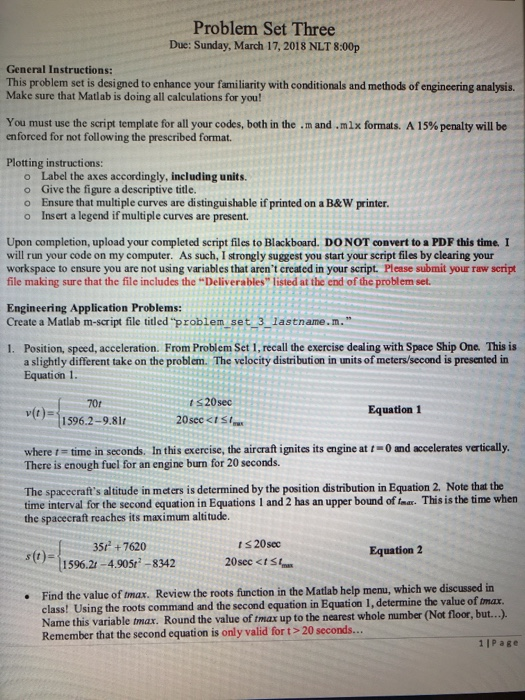
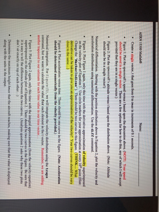
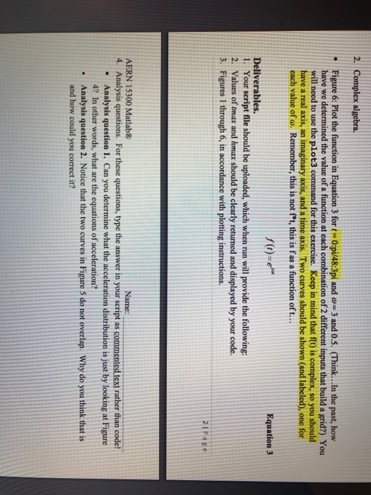
Problem Set Three Due: Sunday, March 17,2018 NLT 8:00p General Instructions: This problem set is designed to enhance your familiarity with conditionals and methods of engineering analysis. Make sure that Matlab is doing all calculations for you! You must use the script template for all your codes, both in the . m and .m1x formats. A 15% penalty will be enforced for not following the prescribed format. Plotting instructions: o Label the axes accordingly, including units o Give the figure a descriptive title. o Ensure that multiple curves are distinguishable if printed on a B&W printer. o Insert a legend if multiple curves are present. Upon completion, upload your completed script files to Blackboard. DO NOT convert to a PDF this time. I will run your code on my computer. As such, I strongly suggest you start your script files by clearing your workspace to ensure you are not using variables that aren't created in your script. Please submit your raw seript file making sure that the file includes the Deliverables" listed at the end of the problem set. Engineering Application Problems: Create a Matlab m-script file titled "problem set 3lastname.m. Position, speed, acceleration. From Problem Set I, recall the exercise dealing with Space Ship One. This is a slightly different take on the problem. The velocity distributi on in units of meters/second is presented in Equation 1. 1. t S20sec v(t) 70r 1596.2-9.81t Equation 1 where t time in seconds. In this exercise, the aircraft ignites its engine at t-0 and accelerates vertically. There is enough fuel for an engine burn for 20 seconds. The spacecraft's altitude in meters is determined by the position distribution in Equation 2. Note that the time interval for the second equation in Equations 1 and 2 has an upper bound of far. This is the time when the spacecraft reaches its maximum altitude. 35r +7620 1596.21-4.905t-8342 t S 20sec s(t)- Equation 2 Review the roots function in the Matlab help menu, which we discussed in Find the value of tmax. class! Using the roots command and the second equation in Equation I, determine the value of max Name this variable tmax. Round th . e value of tmax up to the nearest whole number (Not floor, but...). Remember that the second equation is only valid for t > 20 seconds 1IPage AERN i 5300 Matlab Name Create a single vector, t that goes from 0 to tmax in increments of 0.1 seconds. Figure 1: Plot the spacecraft's speed versus t based upon the discussion above. (NOTE: Your speed should be saved in a single vector. There are a few options for how to do this, any of which I will accept provided that they are in a single vector.) Figure 2: Plot the spacecraft's altitude versus t based upon the distribution above. (Note: Altitude should also be in a single vector!) Numerical differentiation. Starting with the position distribution above in Equation 2, plot the velocity and acceleration distributions using numerical differentiation. Use the diff command. Figure 3: Plot Figure 1 again, only this time with the derivative approximation of velocity superimposed on the velocity plot of Equation 1. Use circle markers for your approximation at every 10th point (Hint: Change the MarkerIndices'). There should be two curves in this figure. (THINK... What derivative can be taken to give you an approximation of the velocity? Your two curves should be very close to the same...) Figure 4: Plot acceleration versus time. There should be one curve in the figure. (Note: Acceleration should be determined numerically from the velocity provided.) Numerical integration. For figure (5), we will integrate the velocity distribution using the trapz command, but we want to calculate the value for each element in the t vector. Remember, we are adding another trapezoid to our estimate for each time value in our time vector Figure 5: Plot Figure 2 again, only this time with the integral approximation (from the velocity equation) on the altitude plot of Equation 2. There should be two curves in the figure. Be sure that it is easy to tell the difference between the two curves. (Analysis question 2 asks why these two plots don't sit exactly on top of each other...) Determine the maximum height hmax that the aircraft reaches, making sure that the value is displayed along with the units in the output. 2. Complex algebra Figure 6: Plot the function in Equation 3 for tH0:pi/48:3pi and o-3 and O.S. (Think...In the past, how have we determined the value of a function at each combination of 2 different inputs that build a grid?) You will need to use the plot3 command for this exercise. Keep in mind that f(t) is complex, so you should have a real axis, an imaginary axis, and a time axis. Two curves should be shown (and labeled), one for each value of w. Equation 3 Deliverables. 1. Your script file should be uploaded, which when run will provide the following 2. Values of tmar and hmar should be clearly returned and displayed by your code. 3. Figures 1 through 6, in accordance with plotting instructions AERN 15300 Matlab 4 Analysis questions. For these questions, type the answer in your script as commented text rather than code Analysis question 1. Can you determine what the acceleration distribution is just by looking at Figure 4? In other words, what are the equations of acceleration Analysis question 2. Notice that the two curves in Figure 5 do not overlap. Why do you think that is and how could you correct it? . Problem Set Three Due: Sunday, March 17,2018 NLT 8:00p General Instructions: This problem set is designed to enhance your familiarity with conditionals and methods of engineering analysis. Make sure that Matlab is doing all calculations for you! You must use the script template for all your codes, both in the . m and .m1x formats. A 15% penalty will be enforced for not following the prescribed format. Plotting instructions: o Label the axes accordingly, including units o Give the figure a descriptive title. o Ensure that multiple curves are distinguishable if printed on a B&W printer. o Insert a legend if multiple curves are present. Upon completion, upload your completed script files to Blackboard. DO NOT convert to a PDF this time. I will run your code on my computer. As such, I strongly suggest you start your script files by clearing your workspace to ensure you are not using variables that aren't created in your script. Please submit your raw seript file making sure that the file includes the Deliverables" listed at the end of the problem set. Engineering Application Problems: Create a Matlab m-script file titled "problem set 3lastname.m. Position, speed, acceleration. From Problem Set I, recall the exercise dealing with Space Ship One. This is a slightly different take on the problem. The velocity distributi on in units of meters/second is presented in Equation 1. 1. t S20sec v(t) 70r 1596.2-9.81t Equation 1 where t time in seconds. In this exercise, the aircraft ignites its engine at t-0 and accelerates vertically. There is enough fuel for an engine burn for 20 seconds. The spacecraft's altitude in meters is determined by the position distribution in Equation 2. Note that the time interval for the second equation in Equations 1 and 2 has an upper bound of far. This is the time when the spacecraft reaches its maximum altitude. 35r +7620 1596.21-4.905t-8342 t S 20sec s(t)- Equation 2 Review the roots function in the Matlab help menu, which we discussed in Find the value of tmax. class! Using the roots command and the second equation in Equation I, determine the value of max Name this variable tmax. Round th . e value of tmax up to the nearest whole number (Not floor, but...). Remember that the second equation is only valid for t > 20 seconds 1IPage AERN i 5300 Matlab Name Create a single vector, t that goes from 0 to tmax in increments of 0.1 seconds. Figure 1: Plot the spacecraft's speed versus t based upon the discussion above. (NOTE: Your speed should be saved in a single vector. There are a few options for how to do this, any of which I will accept provided that they are in a single vector.) Figure 2: Plot the spacecraft's altitude versus t based upon the distribution above. (Note: Altitude should also be in a single vector!) Numerical differentiation. Starting with the position distribution above in Equation 2, plot the velocity and acceleration distributions using numerical differentiation. Use the diff command. Figure 3: Plot Figure 1 again, only this time with the derivative approximation of velocity superimposed on the velocity plot of Equation 1. Use circle markers for your approximation at every 10th point (Hint: Change the MarkerIndices'). There should be two curves in this figure. (THINK... What derivative can be taken to give you an approximation of the velocity? Your two curves should be very close to the same...) Figure 4: Plot acceleration versus time. There should be one curve in the figure. (Note: Acceleration should be determined numerically from the velocity provided.) Numerical integration. For figure (5), we will integrate the velocity distribution using the trapz command, but we want to calculate the value for each element in the t vector. Remember, we are adding another trapezoid to our estimate for each time value in our time vector Figure 5: Plot Figure 2 again, only this time with the integral approximation (from the velocity equation) on the altitude plot of Equation 2. There should be two curves in the figure. Be sure that it is easy to tell the difference between the two curves. (Analysis question 2 asks why these two plots don't sit exactly on top of each other...) Determine the maximum height hmax that the aircraft reaches, making sure that the value is displayed along with the units in the output. 2. Complex algebra Figure 6: Plot the function in Equation 3 for tH0:pi/48:3pi and o-3 and O.S. (Think...In the past, how have we determined the value of a function at each combination of 2 different inputs that build a grid?) You will need to use the plot3 command for this exercise. Keep in mind that f(t) is complex, so you should have a real axis, an imaginary axis, and a time axis. Two curves should be shown (and labeled), one for each value of w. Equation 3 Deliverables. 1. Your script file should be uploaded, which when run will provide the following 2. Values of tmar and hmar should be clearly returned and displayed by your code. 3. Figures 1 through 6, in accordance with plotting instructions AERN 15300 Matlab 4 Analysis questions. For these questions, type the answer in your script as commented text rather than code Analysis question 1. Can you determine what the acceleration distribution is just by looking at Figure 4? In other words, what are the equations of acceleration Analysis question 2. Notice that the two curves in Figure 5 do not overlap. Why do you think that is and how could you correct it