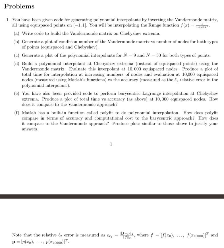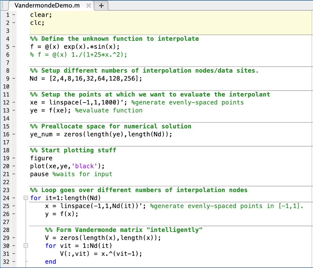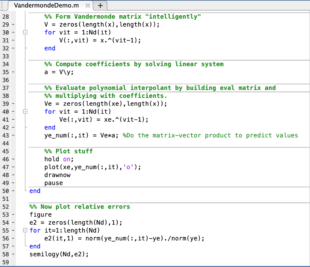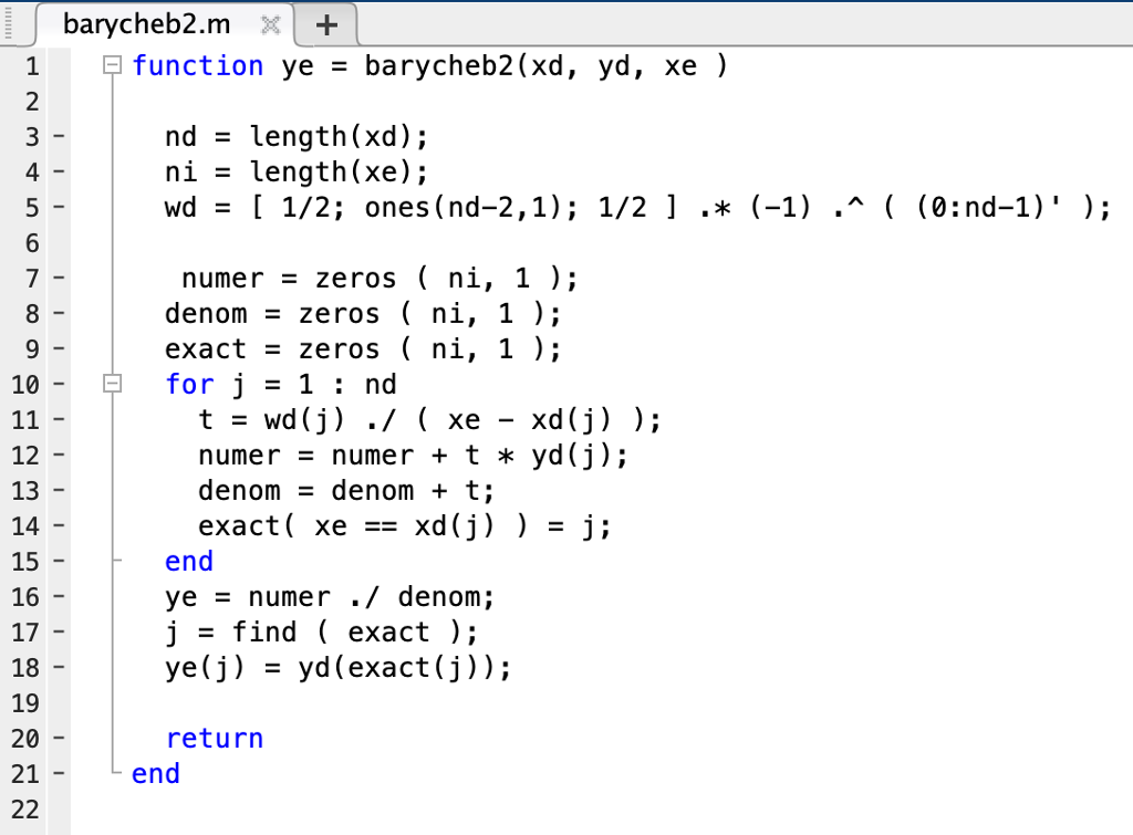
Problems 1. You have been given code for generating polynomial interpolants by inverting the Vandermonde matrix all using equispaced points on 1,1 You will be interpolating the Runge function f(x) (a) Write code to build the Vandermonde matrix on Chebyshev extrema. (b) Generate a plot of condition number of the Vandermonde matrix vs number of nodes for both types of points (equispaced and Chebyshev) (c) Generate a plot of the polynomial interpolants for N 9 and N-50 for both types of points. (d) Build a polynomial interpolant at Chebyshev extrema (instead of equispaced points) using the Vandermonde matrix. Evaluate this interpolant at 10,000 equispaced nodes. Produce a plot of total time for interpolation at increasing numbers of nodes and evaluation at 10,000 equispaced nodes (measured using Matlab's functions) vs the accuracy (measured as the L2 relative error in the polynomial interpolant) (e) You have also been provided code to perform barycentric Lagrange interpolation at Chebyshev extrema. Produce a plot of total time vs accuracy (as above) at 10,000 equispaced nodes. How does it compare to the Vandermonde approach'? (f) Matlab has a built-in function called polyfit to do polynomial interpolation. How does polyfit compare in terms of accuracy and computational cost to the barycentric approach? How does it compare to the Vandermonde approach Produce plots similar to those above to justify your answers where f lf(ro), ..., f(x10000)]7 and Note that the relative error is measured as e- p = [P(zo), . . . , p(x10000)]T. VandermondeDemo.m + clear; clc; 1 %% Define the unknown function to interpolate f -@(x) exp(x).#51n(x); 4 %% Setup different numbers of interpolation nodes/data sites. Nd[2,4,8,16,32,64,128,256]; 10 %% Setup the points at which we want to evaluate the interpolant xe linspace(-1,1, 1000 )'; %generate evenly-spaced points ye f(xe); %evaluate function 12 13 14 15 16 17 18 19 20 21 %% Preallocate space for numerical solution ye_num zeros(length (ye),length (Nd)); start plotting stuff figure plot(xe,ye, 'black'); pause %waits for input %% Loop goes over different numbers of interpolation nodes for it-1: length(Nd) 23 24 25 26 27 28 29 30 31 32 x - linspace(-1,1,Nd(it))'; %generate evenly-spaced points in [-1,1]. y - f(x); %% Form Vandermonde matrix "intelligently" V - zeros(length(x), length(x)); for vit1:Nd (it) V(:,vit) x.(vit-1)1; end VandermondeDemo.m 28 29 30 31 32 %% Form Vandermonde matrix "intelligently" V - zeros(length(x), length(x)); for vit1:Nd (it) end %% Compute coefficients by solving linear system 34 35 36 37 38 39 40 41 42 43 %% Evaluate polynomial interpolant by building eval matrix and %% multiplying with coefficients. Ve - zeros(length(xe),length(x)); for vit1:Nd(it) Ve(:,vit) - xe.~(vit-1); end ye-num(t, it ) -Ve*a ; %Do the matrix-vector product to predict values %% Plot stuff hold on; 45 46 47 48 49 50 51 52 53 54 d rawnow pause end %% Now plot relative errors figure e2 - zeros (length(Nd),1); lfor it-1: length(Nd) 56 57 58 59 e2(it,1)norm(ye_num(:,it)-ye).orm(ye); semilogy (Nd,e2); baryche62.m X1 1 2 3 4 function yebarycheb2(xd, yd, xe ) nd - length (xd); ni - length (xe); wd = [ 1/2; ones(nd-2 , 1); 1/2 ] .* (-1) .^ ( (0:nd-1)' ); numer - zeros ( ni, 1); denom zeros ( ni, 1); exact - zeros ( ni, 1); for j - 1: nd numer - numer t yd(j); denom - denom + t; exact( xe xd(j) )- j; end ye numer ./ denom; j - find ( exact ); ye(j) - yd(exact (j)); return end Problems 1. You have been given code for generating polynomial interpolants by inverting the Vandermonde matrix all using equispaced points on 1,1 You will be interpolating the Runge function f(x) (a) Write code to build the Vandermonde matrix on Chebyshev extrema. (b) Generate a plot of condition number of the Vandermonde matrix vs number of nodes for both types of points (equispaced and Chebyshev) (c) Generate a plot of the polynomial interpolants for N 9 and N-50 for both types of points. (d) Build a polynomial interpolant at Chebyshev extrema (instead of equispaced points) using the Vandermonde matrix. Evaluate this interpolant at 10,000 equispaced nodes. Produce a plot of total time for interpolation at increasing numbers of nodes and evaluation at 10,000 equispaced nodes (measured using Matlab's functions) vs the accuracy (measured as the L2 relative error in the polynomial interpolant) (e) You have also been provided code to perform barycentric Lagrange interpolation at Chebyshev extrema. Produce a plot of total time vs accuracy (as above) at 10,000 equispaced nodes. How does it compare to the Vandermonde approach'? (f) Matlab has a built-in function called polyfit to do polynomial interpolation. How does polyfit compare in terms of accuracy and computational cost to the barycentric approach? How does it compare to the Vandermonde approach Produce plots similar to those above to justify your answers where f lf(ro), ..., f(x10000)]7 and Note that the relative error is measured as e- p = [P(zo), . . . , p(x10000)]T. VandermondeDemo.m + clear; clc; 1 %% Define the unknown function to interpolate f -@(x) exp(x).#51n(x); 4 %% Setup different numbers of interpolation nodes/data sites. Nd[2,4,8,16,32,64,128,256]; 10 %% Setup the points at which we want to evaluate the interpolant xe linspace(-1,1, 1000 )'; %generate evenly-spaced points ye f(xe); %evaluate function 12 13 14 15 16 17 18 19 20 21 %% Preallocate space for numerical solution ye_num zeros(length (ye),length (Nd)); start plotting stuff figure plot(xe,ye, 'black'); pause %waits for input %% Loop goes over different numbers of interpolation nodes for it-1: length(Nd) 23 24 25 26 27 28 29 30 31 32 x - linspace(-1,1,Nd(it))'; %generate evenly-spaced points in [-1,1]. y - f(x); %% Form Vandermonde matrix "intelligently" V - zeros(length(x), length(x)); for vit1:Nd (it) V(:,vit) x.(vit-1)1; end VandermondeDemo.m 28 29 30 31 32 %% Form Vandermonde matrix "intelligently" V - zeros(length(x), length(x)); for vit1:Nd (it) end %% Compute coefficients by solving linear system 34 35 36 37 38 39 40 41 42 43 %% Evaluate polynomial interpolant by building eval matrix and %% multiplying with coefficients. Ve - zeros(length(xe),length(x)); for vit1:Nd(it) Ve(:,vit) - xe.~(vit-1); end ye-num(t, it ) -Ve*a ; %Do the matrix-vector product to predict values %% Plot stuff hold on; 45 46 47 48 49 50 51 52 53 54 d rawnow pause end %% Now plot relative errors figure e2 - zeros (length(Nd),1); lfor it-1: length(Nd) 56 57 58 59 e2(it,1)norm(ye_num(:,it)-ye).orm(ye); semilogy (Nd,e2); baryche62.m X1 1 2 3 4 function yebarycheb2(xd, yd, xe ) nd - length (xd); ni - length (xe); wd = [ 1/2; ones(nd-2 , 1); 1/2 ] .* (-1) .^ ( (0:nd-1)' ); numer - zeros ( ni, 1); denom zeros ( ni, 1); exact - zeros ( ni, 1); for j - 1: nd numer - numer t yd(j); denom - denom + t; exact( xe xd(j) )- j; end ye numer ./ denom; j - find ( exact ); ye(j) - yd(exact (j)); return end