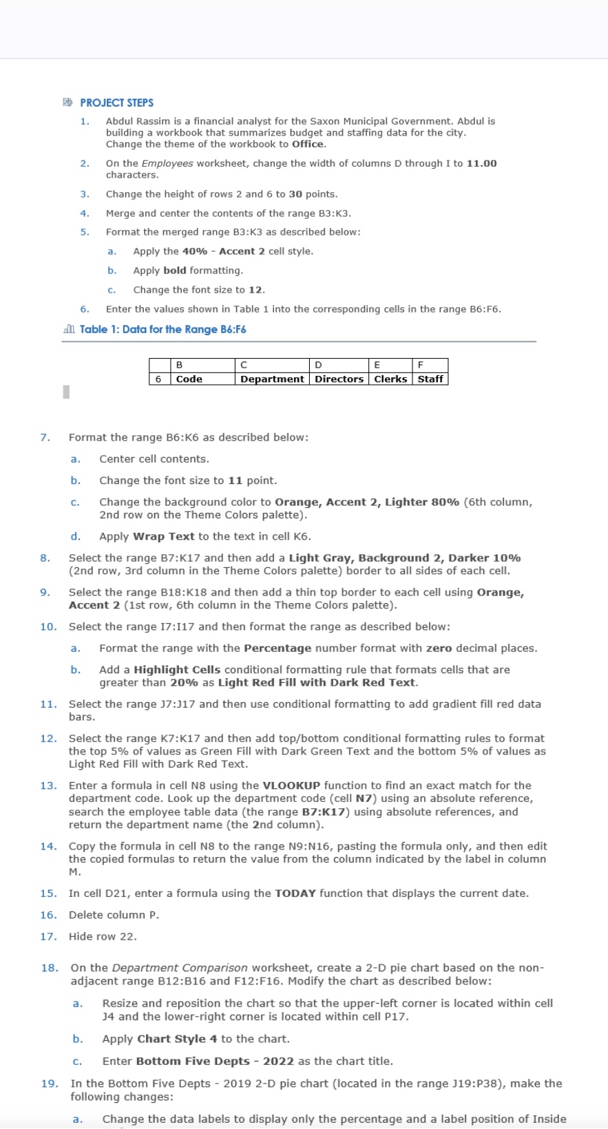
PROJECT STEPS

Abdul Rassim is a financial analyst for the Saxon Municipal Government. Abdul is building a workbook that summarizes budget and staffing data for the city. Change the theme of the workbook to Office.

On the Employees worksheet, change the width of columns D through I to $11\mathrm{.}00$ characters.

Change the height of rows $2$ and $6$ to $30$ points.

Merge and center the contents of the range B$3$:K$3.$

Format the merged range B$3$:K$3$ as described below:

a$.$ Apply the $40\%-$ Accent $2$ cell style.

b$.$ Apply bold formatting.

c$.$ Change the font size to $12.$

Enter the values shown in Table $1$ into the corresponding cells in the range B$6$:F$6.$

In Table $1$: Data for the Range B$6$:F$6$

$\backslash$table$[[,$B$,$C$,$D$,$E$,$F$],[6,$Code,Department,Directors,Clerks,Staff$]]$

Format the range B$6$:K$6$ as described below:

a$.$ Center cell contents.

b$.$ Change the font size to $11$ point.

c$.$ Change the background color to Orange, Accent $2,$ Lighter $80\%(6$ th column, $2$nd row on the Theme Colors palette$).$

d$.$ Apply Wrap Text to the text in cell K$6.$

Select the range B$7$:K$17$ and then add a Light Gray, Background $2,$ Darker $10\%(2$nd row, $3$rd column in the Theme Colors palette$)$ border to all sides of each cell.

Select the range B$18$:K$18$ and then add a thin top border to each cell using Orange, Accent $2(1$st row, $6$ th column in the Theme Colors palette$).$

Select the range I$7$:I$17$ and then format the range as described below:

a$.$ Format the range with the Percentage number format with zero decimal places.

b$.$ Add a Highlight Cells conditional formatting rule that formats cells that are greater than $20\%$ as Light Red Fill with Dark Red Text.

Select the range $J7$:$J17$ and then use conditional formatting to add gradient fill red data bars.

Select the range K$7$:K$17$ and then add top$/$bottom conditional formatting rules to format the top $5\%$ of values as Green Fill with Dark Green Text and the bottom $5\%$ of values as Light Red Fill with Dark Red Text.

Enter a formula in cell N$8$ using the VLOOKUP function to find an exact match for the department code. Look up the department code $($cell N$7)$ using an absolute reference, search the employee table data $($the range B$7$:K$17)$ using absolute references, and return the department name $($the $2$ nd column$).$

Copy the formula in cell N$8$ to the range N$9$:N$16,$ pasting the formula only, and then edit the copied formulas to return the value from the column indicated by the label in column M$.$

In cell D$21,$ enter a formula using the TODAY function that displays the current date.

Delete column $P.$

Hide row $22.$

On the Department Comparison worksheet, create a $2-$D pie chart based on the nonadjacent range B$12$:B$16$ and F$12$:F$16.$ Modify the chart as described below:

a$.$ Resize and reposition the chart so that the upper$-$left corner is located within cell J$4$ and the lower$-$right corner is located within cell P$17.$

b$.$ Apply Chart Style $4$ to the chart.

c$.$ Enter Bottom Five Depts $-2022$ as the chart title.

In the Bottom Five Depts $-20192-$D pie chart $($located in the range J$19$:P$38),$ make the following changes:

a$.$ Change the data labels to display only the percentage and a label position of Inside