PROJECT STEPS

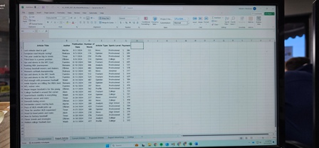
1. Jack Roscoe started running a sports blog two years ago, and since then, it has provided a second income for him and his family. Jack is reviewing the recent articles written for the blog along with the payments to the authors and the income from ads. He asks for your help in using Excel tables to analyze the data. Go to the August Articles worksheet, which lists the articles published in August 2024. Create a table as follows so that Jack can summarize and filter the data and display articles with the highest payment amounts:
   1. Format the August articles data (range A1:G26) as a table using Aqua, Table Style Medium 5.
   2. Use AugArticles as the name of the table.
   3. Filter the table using a custom AutoFilter to display projects with a Payment amount greater than or equal to $500.
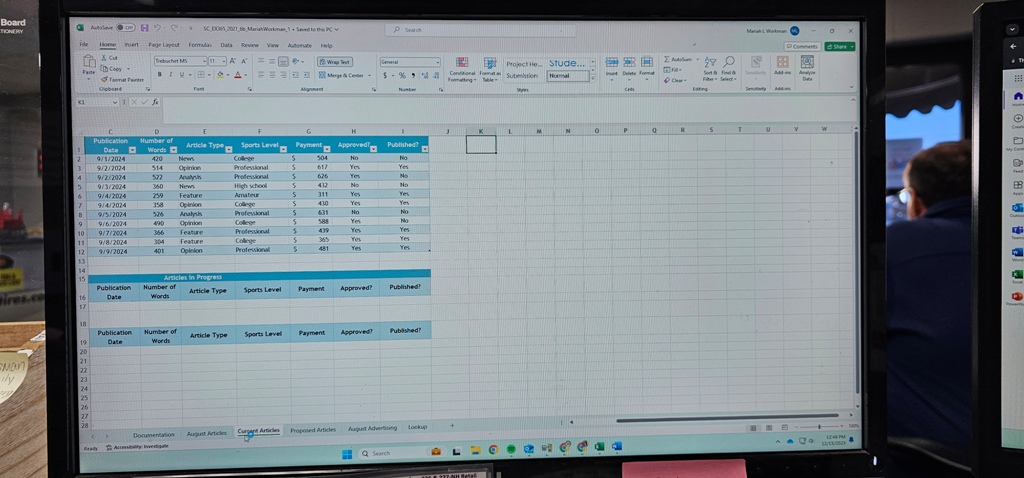
2. Go to the Current Articles worksheet, which contains the CurrentArticles table listing articles that are scheduled for publication during the first 10 days in September. Jack received a proposal for a new article that he wants to publish on September 10. Insert a row to the end of the CurrentArticles table for a new record containing the data shown in Table 1.

Table 1: New Record for the CurrentArticles Table

Article Title	Author	Publication Date	Number of Words	Article Type	Sports Level	Payment	Approved?	Published?
Weekend preview	Aken	9/10/2024	482	News	College	$578	Yes	No

1. Sort the CurrentArticles table in descending order by payment amount so that Jack can quickly track the payments for each article.
2. Jack wants to list the published articles in a separate part of the worksheet. Use an advanced filter as follows to list these articles in a new range:
   1. In cell I18, type Yes as the value to filter on in the criteria range.
   2. Create an advanced filter using the CurrentArticles table (range A1:I13) as the List range.
   3. Use the range A17:I18 as the Criteria range.
   4. Copy the results to another location, starting in the range A20:I20.
3. As a contrast, Jack also wants to list the projects that are not in development. In the CurrentArticles table, display the filter arrows, and then filter the table to display the articles that have not been published yet. (Hint: If the Filter Button check box is not available, remove and then redisplay the header row.)
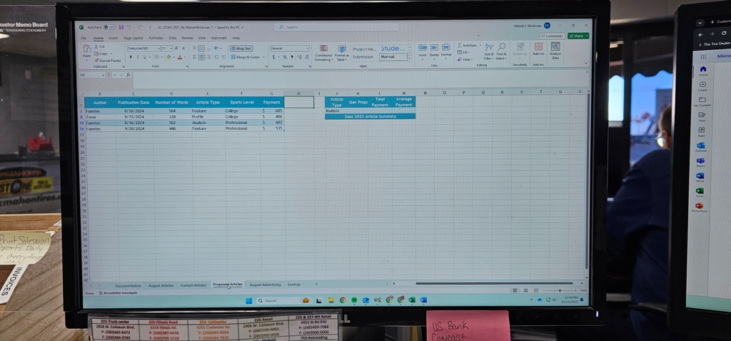
4. Go to the Proposed Articles worksheet, which lists articles that have been proposed for publication in September. Jack suspects the ProposedArticles table has a duplicate record. Identify the duplicate as follows:
   1. Clear the filter from the ProposedArticles table to display all the records.
   2. In the range A2:A16, create a Conditional Formatting Highlight Cells Rule that displays cells with duplicate values using Light Red Fill with Dark Red Text.
   3. Delete the second instance of the duplicate record so that you can summarize the data accurately.
5. Jack includes photos with all articles, but he asks a graphic artist to create additional illustrations such as charts and infographics for feature stories longer than 400 words. Add a column to the ProposedArticles table, and determine which articles meet the criteria as follows:
   1. In cell H1, type Extra Art as the column heading.
   2. In cell H2, enter a formula using the AND function that includes structured references to display TRUE if an article has a [@[Number of Words]] value >400 and an [@[Article Type]] of "Feature". Fill the range H3:H15 with the formula in cell H2 if Excel does not do so automatically.
6. Add a Total Row to the ProposedArticles table, which automatically counts the number of Extra Art values. Using the total row, display the sum of the payment amounts.
7. Jack asks you to identify the articles that contain 500 words or more, those that contain 400 words or more, and those that contain less than 400 words.
   1. In the Number of Words column (range D2:D15), create a new Icon Set Conditional Formatting rule using the 3 Traffic Lights (Rimmed) icons.
   2. Reverse the icon order.
   3. Display the red traffic light icon in cells with a Number type value greater than or equal to 500.
   4. Display the yellow traffic light icon in cells with a Number type value greater than or equal to 400.
   5. Display the green traffic light icon in cells with a Number type value less than 400.
8. Jack also wants to compare the payment amounts visually. In the Payment column (range G2:G15), create a new Data Bars Conditional Formatting rule using Blue Gradient Fill Data Bars.
9. Wrap the text in cell K1 to display the complete contents of the cell.
10. Jack wants to summarize the number of articles proposed by the article type and calculate their total payment and average payment amounts. Calculate this information for Jack as follows:
    1. In cell K2, enter a formula using the COUNTIF function that counts the number of proposed Analysis articles, using ProposedArticles[Article Type] as the range and cell J2 as the criteria.
    2. Fill the range K3:K6 with the formula in cell K2.
    3. In cell L2, enter a formula using the SUMIF function that totals the payments for proposed Analysis articles, using ProposedArticles[Article Type] as the range, cell J2 as the criteria, and ProposedArticles[Payment] as the sum_range.
    4. Fill the range L3:L6 with the formula in cell L2.
    5. In cell M2, enter a formula using the AVERAGEIF function that averages the payments for proposed Analysis articles, using ProposedArticles[Article Type] as the range, cell J2 as the criteria, and ProposedArticles[Payment] as the average_range.
    6. Fill the range M3:M6 with the formula in cell M2.
11. In the range J9:M14, Jack needs to insert a summary of the proposed and published articles from September 2023. Insert this data as a table as follows:
    1. Insert a table in the range J9:M14, specifying that the data has headers.
    2. In the new table, enter the data shown in Table 2.
    3. AutoFit the contents of columns J:M to display the complete cell contents.
    4. Apply Aqua, Table Style Medium 5 to the new table to match the formatting of the ProposedArticles table.

Table 2: Data for the New Table

Article Type	Proposed	Published	Payment
Analysis	5	3	1,998
Feature	5	4	2,065
News	4	3	1,603
Opinion	3	3	1,512
Profile	3	2	1,004

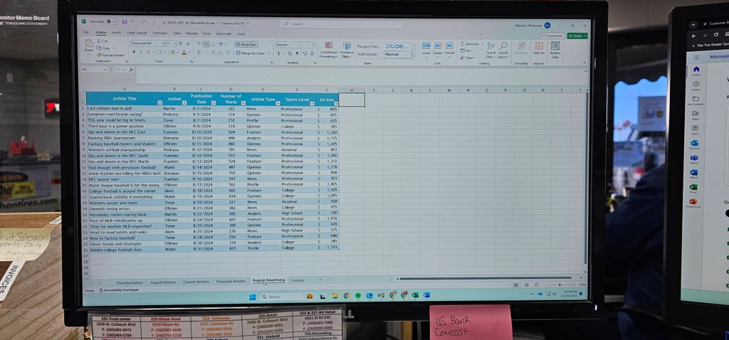
1. Go to the August Advertising worksheet, which lists all the articles published in August. Jack wants to display the data by article type and then list the projects by publication date. Sort the data in the table in ascending order first by article type and then by publication date.
2. Jack also wants to calculate ad amount subtotals for each article type:
   1. Convert the table to a range.
   2. Insert a subtotal at each change in the Article Type value.
   3. Use the Sum function to calculate the subtotals.
   4. Add subtotals to the Ad Amt values only.
   5. Include a summary below the data.
   6. Collapse the outline to display only the subtotals for each article type and the grand total.
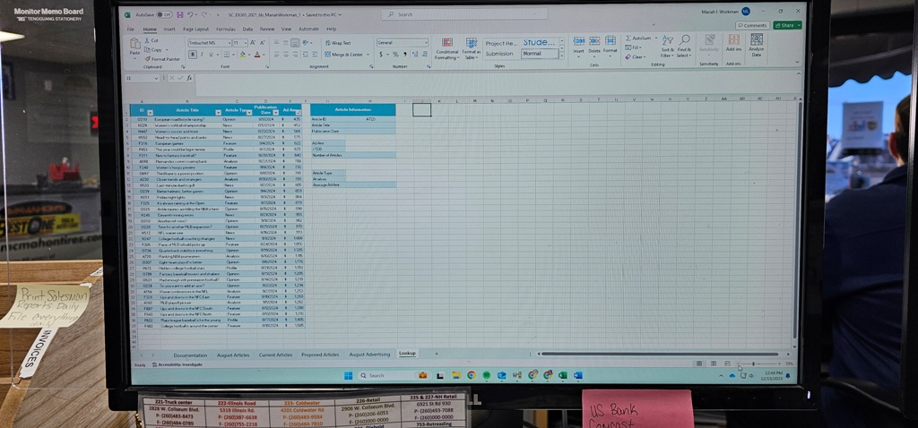
3. Go to the Lookup worksheet, which lists article details, including the ID code that Jack uses to refer to the articles. He wants to find a simple way to look up an article title name based on its ID. Create a formula that provides this information as follows:
   1. In cell H3, begin to enter a formula using the VLOOKUP function.
   2. Use the Article ID (cell H2) as the lookup value.
   3. Use the Lookup table (range A2:E37) as the table_array.
   4. Use the Article Title column (column 2) as the col_index_num.
   5. Specify an exact match (FALSE) for the range_lookup.
4. Jack also wants to look up the publication date of each article. Instead of using the VLOOKUP function, he suggests using the INDEX and MATCH functions, which are faster with large amounts of data. Create a formula that provides the publication date of an article as follows:
   1. In cell H4, begin to enter a formula using the INDEX function.
   2. Use the Lookup table (range A2:E37) as the array.
   3. For the row_num argument, use the MATCH function.
   4. Use the Article ID (cell H2) as the lookup_value for the MATCH function.
   5. Use the ID column (range A2:A37) as the lookup_array for the MATCH function.
   6. Specify an exact match (0) for the MATCH function.
   7. Use the Publication Date column (column 4) as the column_num for the INDEX function.
5. Jack also wants to identify the number of articles that earned more than $500 of advertising and calculate the average ad amount for Analysis articles. Create formulas that provide this information as follows:
   1. In cell H8, create a formula using the DCOUNT function to count the number of articles with ad amounts more than $500, using the Lookup table (range A1:E37) as the database, "Ad Amt" as the field, and the range G6:G7 as the criteria.
   2. In cell H13, create a formula using the DAVERAGE function to average the ad amounts for Analysis articles, using the Lookup table (range A1:E37) as the database, "Ad Amt" as the field, and the range G11:G12 as the criteria.