Provide step by step solutions to these

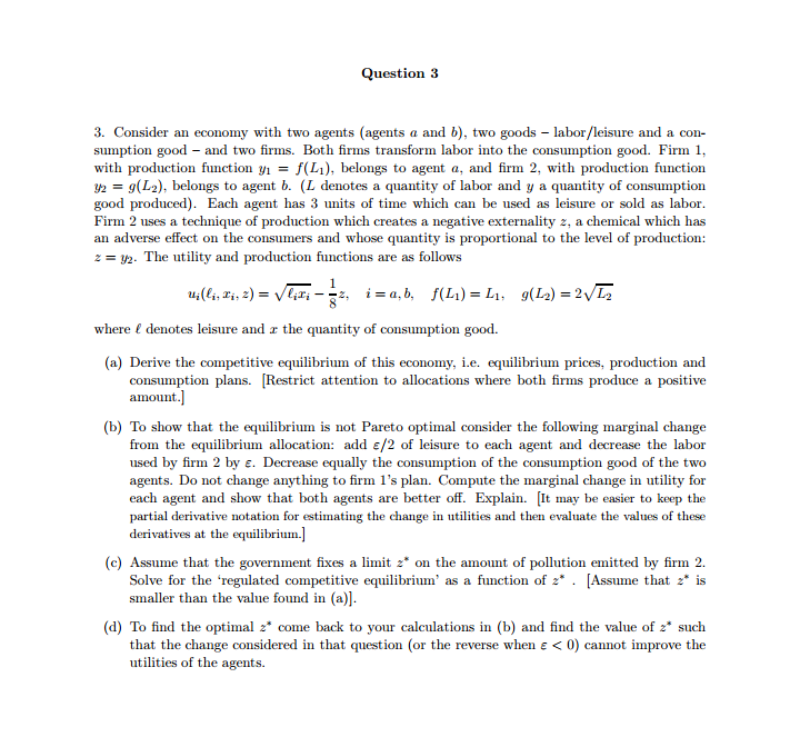
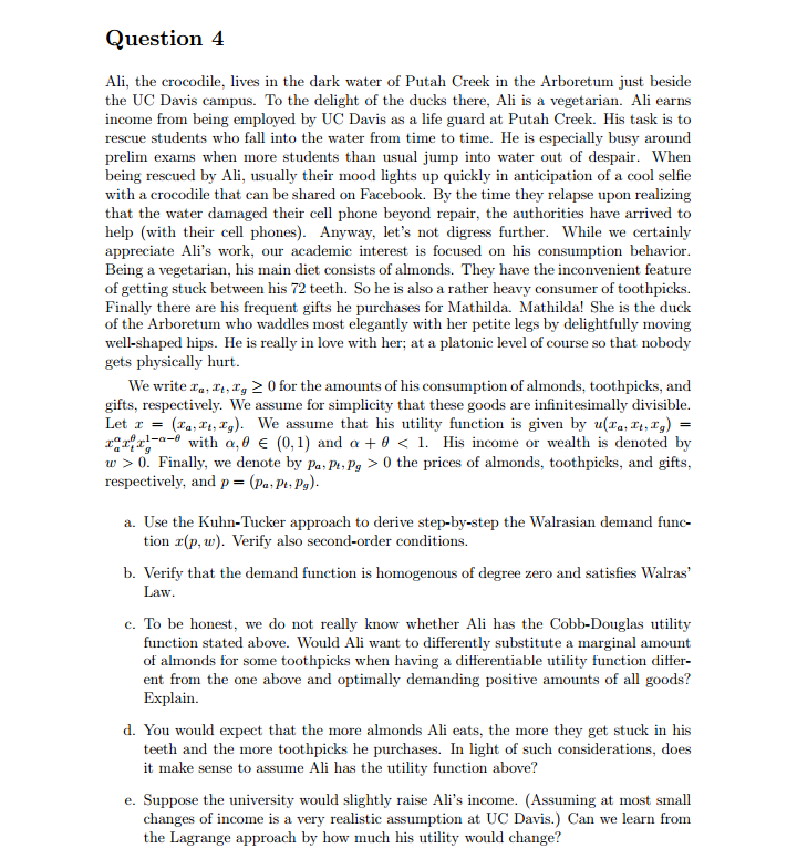
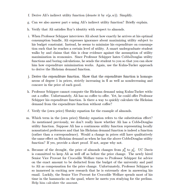
Question 3 3. Consider an economy with two agents (agents a and b), two goods - labor/leisure and a con- sumption good - and two firms. Both firms transform labor into the consumption good. Firm 1, with production function y1 = f(Li), belongs to agent a, and firm 2, with production function 32 = g(L2), belongs to agent b. (L denotes a quantity of labor and y a quantity of consumption good produced). Each agent has 3 units of time which can be used as leisure or sold as labor. Firm 2 uses a technique of production which creates a negative externality =, a chemical which has an adverse effect on the consumers and whose quantity is proportional to the level of production: 2 = 12. The utility and production functions are as follows "(fix,=) =Vir -2, i=ab, f(L) = L. g(12) =2VL2 where f denotes leisure and a the quantity of consumption good. (a) Derive the competitive equilibrium of this economy, i.e. equilibrium prices, production and consumption plans. Restrict attention to allocations where both firms produce a positive amount.] (b) To show that the equilibrium is not Pareto optimal consider the following marginal change from the equilibrium allocation: add z/2 of leisure to each agent and decrease the labor used by firm 2 by z. Decrease equally the consumption of the consumption good of the two agents. Do not change anything to firm 1's plan. Compute the marginal change in utility for each agent and show that both agents are better off. Explain. [It may be easier to keep the partial derivative notation for estimating the change in utilities and then evaluate the values of these derivatives at the equilibrium.] (c) Assume that the government fixes a limit 2* on the amount of pollution emitted by firm 2. Solve for the 'regulated competitive equilibrium' as a function of 2* . [Assume that 2* is smaller than the value found in (a)]. (d) To find the optimal 2* come back to your calculations in (b) and find the value of 2* such that the change considered in that question (or the reverse when 0. Finally, we denote by Pa, Pa, P, > 0 the prices of almonds, toothpicks, and gifts, respectively, and p = (Pa; Pt; Pg). a. Use the Kuhn-Tucker approach to derive step-by-step the Walrasian demand func- tion r(p, w). Verify also second-order conditions. b. Verify that the demand function is homogenous of degree zero and satisfies Walras' Law. c. To be honest, we do not really know whether Ali has the Cobb-Douglas utility function stated above. Would Ali want to differently substitute a marginal amount of almonds for some toothpicks when having a differentiable utility function differ- ent from the one above and optimally demanding positive amounts of all goods? Explain. d. You would expect that the more almonds Ali eats, the more they get stuck in his teeth and the more toothpicks he purchases. In light of such considerations, does it make sense to assume Ali has the utility function above? e. Suppose the university would slightly raise Ali's income. (Assuming at most small changes of income is a very realistic assumption at UC Davis.) Can we learn from the Lagrange approach by how much his utility would change?f. Derive Ali's indirect utility function (denote it by v(p, w)). Simplify. g. Can we also answer part e using Ali's indirect utility function? Briefly explain. h. Verify that Ali satisfies Roy's identity with respect to almonds. i. When Professor Schipper interviews Ali about how exactly he arrives at his optimal consumption bundle, Ali expresses ignorance about maximizing utility subject to his budget constraint. Instead, he seems to minimize his expenditure on consump- tion such that he reaches a certain level of utility. A smart undergraduate student walks by and claims that this is clear evidence against the assumption of utility maximization in economics. Since Professor Schipper hates Cobb-Douglas utility functions and boring calculations, he sends the student to you so that you can show him how expenditure minimization works. Again, use the Kuhn-Tucker approach to derive the Hicksian demand function. j. Derive the expenditure function. Show that the expenditure function is homoge- neous of degree 1 in prices, strictly increasing in a as well as nondecreasing and concave in the price of each good. k. Professor Schipper cannot compute the Hicksian demand using Kuhn-Tucker with- out a coffee. Unfortunately, Ali has no coffee to offer. Yet, he could offer Professor Schipper his expenditure function. Is there a way to quickly calculate the Hicksian demand from the expenditure function without coffee? (. Verify the (own price) Slutsky equation for the example of almonds. m. Which term in the (own price) Slutsky equation refers to the substitution effect? As mentioned previously, we don't really know whether Ali has a Cobb-Douglas utility function. Suppose Ali has a continuous utility function representing locally nonsatiated preferences and that his Hicksian demand function is indeed a function (rather than a correspondence). Would a change in prices still have qualitatively the same effect on Hicksian demand as when he has the above Cobb-Douglas utility function? If yes, provide a short proof. If not, argue why not. n. Because of the drought, the price of almonds changes from pa to pa- UC Davis is committed to keep Ali as well off as before the price change. The newly hired Senior Vice Provost for Crocodile Welfare turns to Professor Schipper for advice on the exact amount to be deducted from the budget of the university and paid to Ali as compensation for the price change. Unfortunately, Professor Schipper is so immersed in exciting new research that he is extremely slow in answering his email. Luckily, the Senior Vice Provost for Crocodile Welfare spends most of his time in the hammocks on the quad, where he meets you studying for the prelims. Help him calculate the amount