Python Please

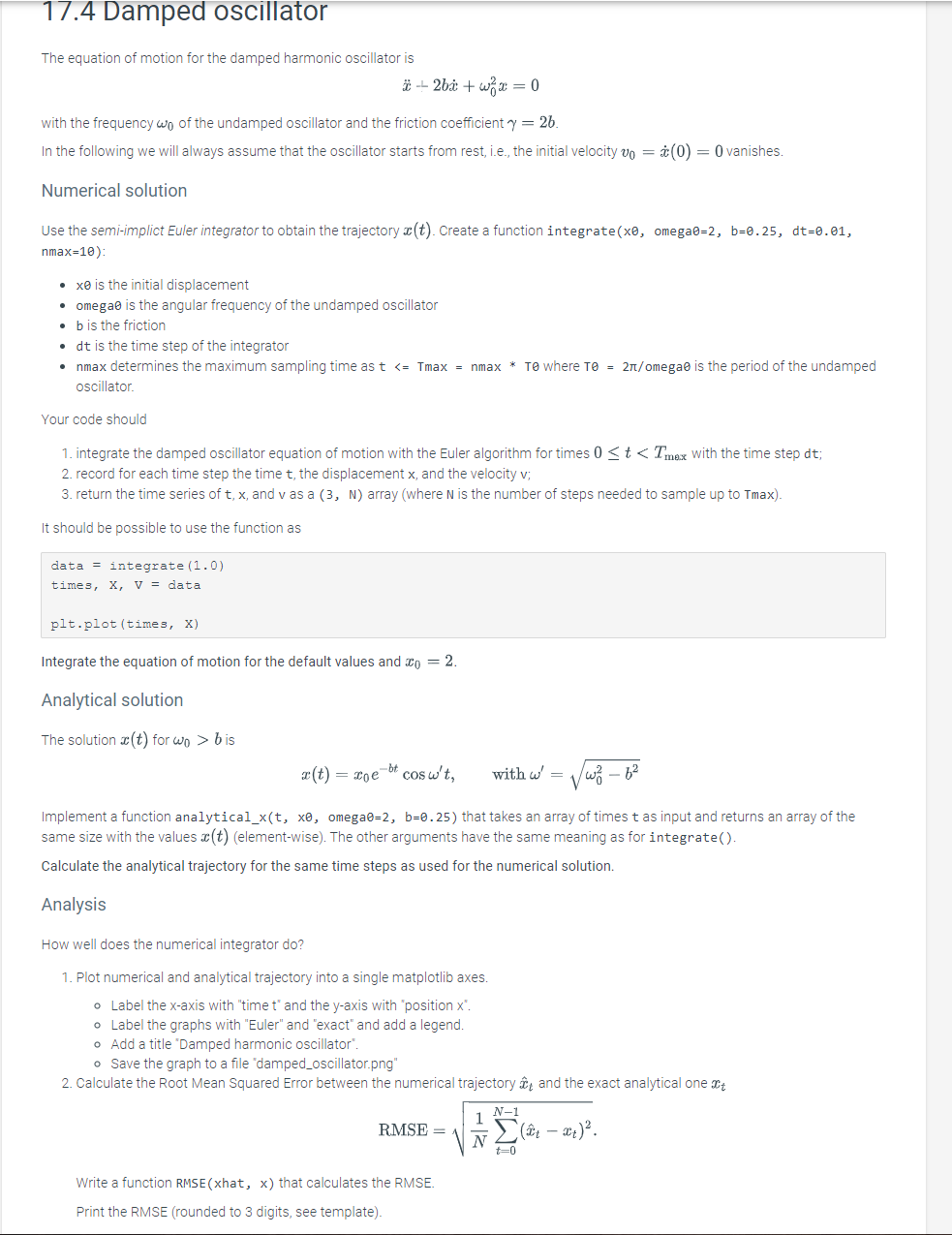
17.4 Damped oscillator The equation of motion for the damped harmonic oscillator is 3 -- 261 + wax = 0 with the frequency wo of the undamped oscillator and the friction coefficient y = 26. In the following we will always assume that the oscillator starts from rest, i.e., the initial velocity vo = c(0) = 0 vanishes. Numerical solution Use the semi-implict Euler integrator to obtain the trajectory c(t). Create a function integrate(xo, omegab=2, b=0.25, dt=0.01, nmax=10): xo is the initial displacement omega is the angular frequency of the undamped oscillator b is the friction dt is the time step of the integrator nmax determines the maximum sampling time as t bis (t) = Doeb cosw't, with w' = vw Implement a function analytical_x(t, xo, omegae=2, b=0.25) that takes an array of times t as input and returns an array of the same size with the values c(t) (element-wise). The other arguments have the same meaning as for integrate(). Calculate the analytical trajectory for the same time steps as used for the numerical solution. Analysis How well does the numerical integrator do? 1. Plot numerical and analytical trajectory into a single matplotlib axes. o Label the x-axis with "timet' and the y-axis with 'position x. o Label the graphs with "Euler" and "exact" and add a legend. o Add a title Damped harmonic oscillator". o Save the graph to a file damped_oscillator.png" 2. Calculate the Root Mean Squared Error between the numerical trajectory it and the exact analytical one It N-1 RMSE= t 2). Write a function RMSE(xhat, x) that calculates the RMSE. Print the RMSE (rounded to 3 digits, see template). 17.4 Damped oscillator The equation of motion for the damped harmonic oscillator is 3 -- 261 + wax = 0 with the frequency wo of the undamped oscillator and the friction coefficient y = 26. In the following we will always assume that the oscillator starts from rest, i.e., the initial velocity vo = c(0) = 0 vanishes. Numerical solution Use the semi-implict Euler integrator to obtain the trajectory c(t). Create a function integrate(xo, omegab=2, b=0.25, dt=0.01, nmax=10): xo is the initial displacement omega is the angular frequency of the undamped oscillator b is the friction dt is the time step of the integrator nmax determines the maximum sampling time as t bis (t) = Doeb cosw't, with w' = vw Implement a function analytical_x(t, xo, omegae=2, b=0.25) that takes an array of times t as input and returns an array of the same size with the values c(t) (element-wise). The other arguments have the same meaning as for integrate(). Calculate the analytical trajectory for the same time steps as used for the numerical solution. Analysis How well does the numerical integrator do? 1. Plot numerical and analytical trajectory into a single matplotlib axes. o Label the x-axis with "timet' and the y-axis with 'position x. o Label the graphs with "Euler" and "exact" and add a legend. o Add a title Damped harmonic oscillator". o Save the graph to a file damped_oscillator.png" 2. Calculate the Root Mean Squared Error between the numerical trajectory it and the exact analytical one It N-1 RMSE= t 2). Write a function RMSE(xhat, x) that calculates the RMSE. Print the RMSE (rounded to 3 digits, see template)