python project any help appreciated

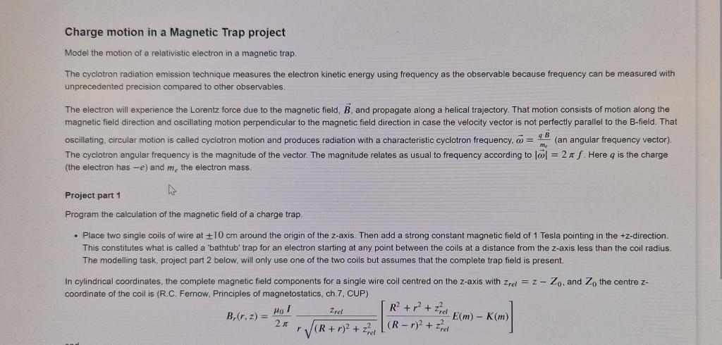
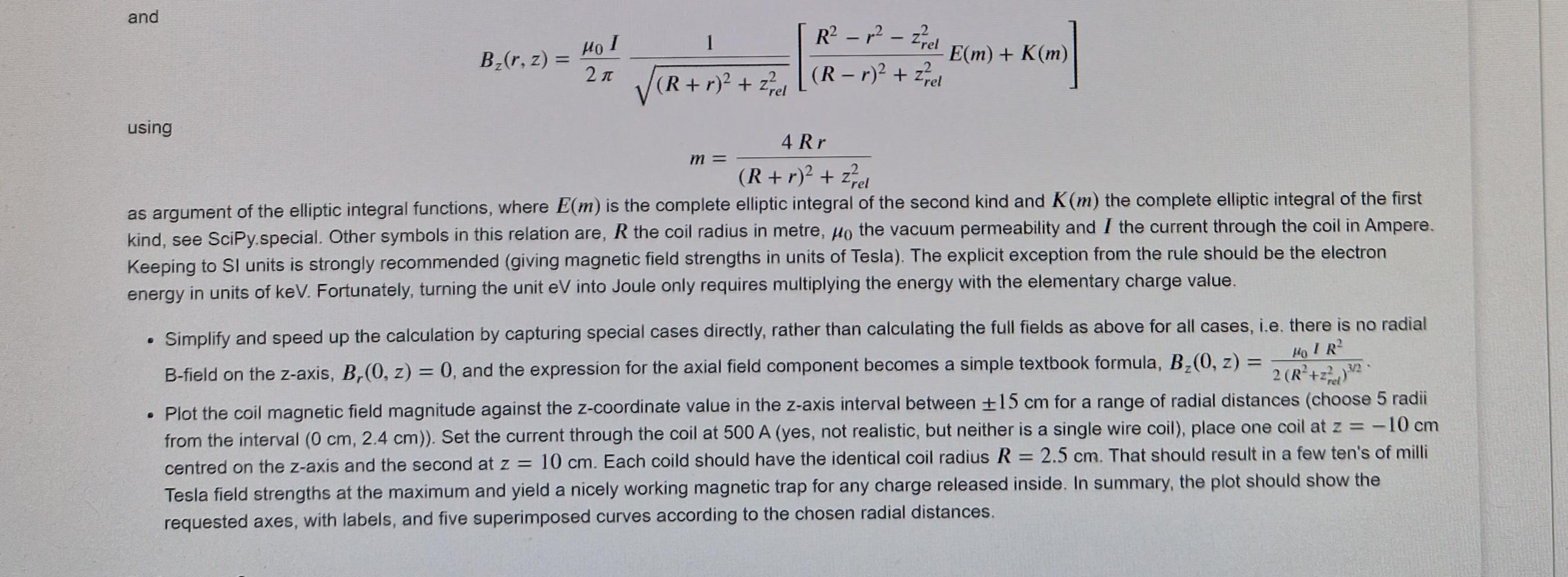
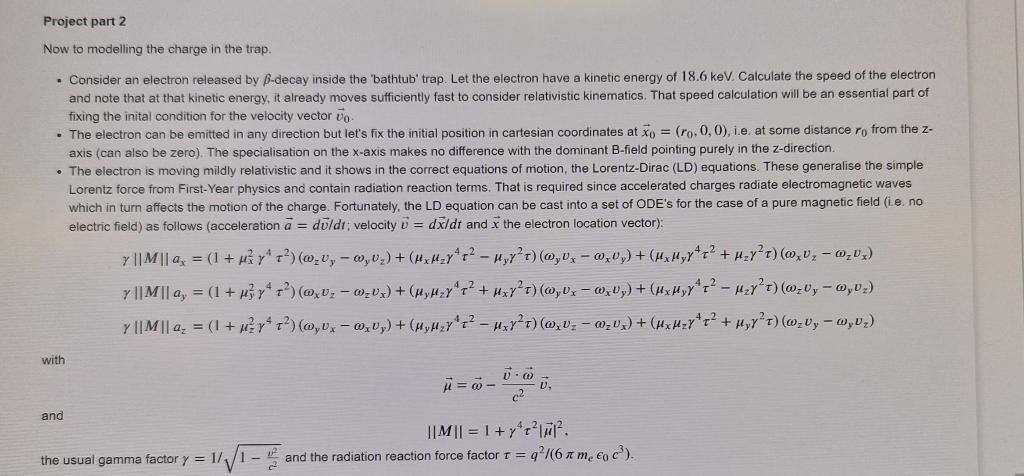
Charge motion in a Magnetic Trap project Model the motion of a relativistic electron in a magnetic trap. The cyclotron radiation emission technique measures the electron kinetic energy using frequency as the observable because frequency can be measured with unprecedented precision compared to other observables. The electron will experience the Lorentz force due to the magnetic field, B, and propagate along a helical trajectory. That motion consists of motion along the magnetic field direction and oscillating motion perpendicular to the magnetic field direction in case the velocity vector is not perfectly parallel to the B-field. That oscillating, circular motion is called cyclotron motion and produces radiation with a characteristic cyclotron frequency, =meqB (an angular frequency vector). The cyclotron angular frequency is the magnitude of the vector. The magnitude relates as usual to frequency according to =2f. Here q is the charge (the electron has e ) and me the electron mass. Project part 1 Program the calculation of the magnetic field of a charge trap. - Place two single coils of wire at 10cm around the origin of the z-axis. Then add a strong constant magnetic field of 1 Tesla pointing in the +z-direction. This constitutes what is called a 'bathtub' trap for an electron starting at any point between the coils at a distance from the z-axis less than the coil radius. The modelling task, project part 2 below, will only use one of the two coils but assumes that the complete trap field is present. In cylindrical coordinates, the complete magnetic field components for a single wire coil centred on the z-axis with zrel=zco - Z0, and Z0 the centre z coordinate of the coil is (R.C. Fernow, Principles of magnetostatics, ch.7, CUP) Br(r,z)=20Ir(R+r)2+zrel2zrel[(Rr)2+zrel2R2+r2+zrel2E(m)K(m)] and Bz(r,z)=20I(R+r)2+zrel21[(Rr)2+zrel2R2r2zrel2E(m)+K(m)] using m=(R+r)2+zrel24Rr as argument of the elliptic integral functions, where E(m) is the complete elliptic integral of the second kind and K ( m ) the complete elliptic integral of the first kind, see SciPy.special. Other symbols in this relation are, R the coil radius in metre, 0 the vacuum permeability and I the current through the coil in Ampere. Keeping to SI units is strongly recommended (giving magnetic field strengths in units of Tesla). The explicit exception from the rule should be the electron energy in units of keV. Fortunately, turning the unit eV into Joule only requires multiplying the energy with the elementary charge value. - Simplify and speed up the calculation by capturing special cases directly, rather than calculating the full fields as above for all cases, i.e. there is no radial B-field on the z-axis, Br(0,z)=0, and the expression for the axial field component becomes a simple textbook formula, Bz(0,z)=2(R2+zrel2)0IR2. - Plot the coil magnetic field magnitude against the z-coordinate value in the z-axis interval between 15cm for a range of radial distances (choose 5 radii from the interval (0cm,2.4cm )). Set the current through the coil at 500A (yes, not realistic, but neither is a single wire coil), place one coil at z=10 cm centred on the z-axis and the second at z=10cm. Each coild should have the identical coil radius R=2.5cm. That should result in a few ten's of milli Tesla field strengths at the maximum and yield a nicely working magnetic trap for any charge released inside. In summary, the plot should show the requested axes, with labels, and five superimposed curves according to the chosen radial distances. Now to modelling the charge in the trap. - Consider an electron released by -decay inside the 'bathtub' trap. Let the electron have a kinetic energy of 18.6 keV. Calculate the speed of the electron and note that at that kinetic energy, it already moves sufficiently fast to consider relativistic kinematics. That speed calculation will be an essential part of fixing the inital condition for the velocity vector v0. - The electron can be emitted in any direction but let's fix the initial position in cartesian coordinates at x0=(r0,0,0), i.e. at some distance r0 from the z axis (can also be zero). The specialisation on the x-axis makes no difference with the dominant B-field pointing purely in the z-direction. - The electron is moving mildly relativistic and it shows in the correct equations of motion, the Lorentz-Dirac (LD) equations. These generalise the simple Lorentz force from First-Year physics and contain radiation reaction terms. That is required since accelerated charges radiate electromagnetic waves which in turn affects the motion of the charge. Fortunately, the LD equation can be cast into a set of ODE's for the case of a pure magnetic field (i.e. no electric field) as follows (acceleration a=dv/dt; velocity v=dx/dt and x the electron location vector): Max=(1+x242)(zvyyvz)+(xz42y2)(yvxxvy)+(xy42+z2)(xvzzvx)May=(1+y242)(xvzzvx)+(yz42+x2)(yvxxvy)+(xy42z2)(zvyyvz)Maz=(1+z242)(yvxxvy)+(yz42x2)(xvzzvx)+(xz42+y2)(zvyyvz) With =c2vv and M=1+422. the usual gamma factor =1/1c2v2 and the radiation reaction force factor t=q2/(6me0c3). - Solve the LD equations of motion numerically using the SciPy function solve_ivp. The initial condition on the coordinates is given above. You will notice that for most initial conditions on the velocity components, the trap is not closed, i.e. electrons escape beyond the z=10 cm coil. This condion is symmetrical around the origin hence from here on we only consider electron trajectories with respect to a single coil. If an electron bounces back at a single coil, it will do so again at its opposite counterpart. - Note that an initial velocity perpendicular to the z-axis will not propagate the electron towards a coil but it rotates around the origin. There, set the maximum emission angle with respect to the z-axis at 89 degrees. - Likewise, restrict the radial distance to the z-axis for the point of emission to values less than 2.4cm. This is because at the exact coil radius, there is a numerically critical point of the magnetic field at the position of the wire, i.e. at z=10cm and r=R, which you should avoid hence the restriction above. - Scan the available parameter space in emission angle (hence v0 ) and r0 to capture all values leading to electron reflection at a single coil. - For the case of a reflected electron (bouncing) at a coil, determine the frequency (1/(2*return time)) of the bounce for each parameter value pair from above. In case of no bounce, store the frequency as zero in case your parameter scan space contains edge cases showing electrons just escaping the trap. - Plot the bounce frequency against the radial distance and emission angle in a 3D scatter plot with appropriate axis labels. Choose appropriate units for the plot, i.e. frequency units of MHz, angle units of degrees and radial distance units of cm