PYTHON - USE JUPITER NOTEBOOK & SHOW ITS CODE [ ALL THE INFO IS GIVEN }

Please, find below the txt file data to use:

*This file contains information of precipitation per cell and per time. *For each time, 25 values are provided, corresponding to the 25 cells of the discretized basin. * 1 2 3 4 5 * 6 7 8 9 10 *11 12 13 14 15 *16 17 18 19 20 *21 22 23 24 25

******************* P t= 0 0.00 0.00 0.00 0.00 0.00 0.00 0.00 0.00 0.00 0.00 0.00 0.00 0.00 0.00 0.00 0.00 0.00 0.00 0.00 0.00 1.00 0.00 0.00 0.00 0.00 P t= 1 0.00 0.00 0.00 0.00 0.00 0.00 0.00 0.00 0.00 0.00 0.00 0.00 0.00 0.00 0.00 1.00 0.00 0.00 0.00 0.00 2.00 1.00 0.00 0.00 0.00 P t= 2 0.00 0.00 0.00 0.00 0.00 0.00 0.00 0.00 0.00 0.00 1.00 0.00 0.00 0.00 0.00 2.00 1.00 0.00 0.00 0.00 3.00 2.00 1.00 0.00 0.00 P t= 3 0.00 0.00 0.00 0.00 0.00 1.00 0.00 0.00 0.00 0.00 2.00 1.00 0.00 0.00 0.00 3.00 2.00 1.00 0.00 0.00 4.00 3.00 2.00 1.00 0.00 P t= 4 1.00 0.00 0.00 0.00 0.00 2.00 1.00 0.00 0.00 0.00 3.00 2.00 1.00 0.00 0.00 4.00 3.00 2.00 1.00 0.00 5.00 4.00 3.00 2.00 1.00 P t= 5 2.00 1.00 0.00 0.00 0.00 3.00 2.00 1.00 0.00 0.00 4.00 3.00 2.00 1.00 0.00 5.00 4.00 3.00 2.00 1.00 4.00 5.00 4.00 3.00 2.00 P t= 6 3.00 2.00 1.00 0.00 0.00 4.00 3.00 2.00 1.00 0.00 5.00 4.00 3.00 2.00 1.00 4.00 5.00 4.00 3.00 2.00 3.00 4.00 5.00 4.00 3.00 P t= 7 4.00 3.00 2.00 1.00 0.00 5.00 4.00 3.00 2.00 1.00 4.00 5.00 4.00 3.00 2.00 3.00 4.00 5.00 4.00 3.00 2.00 3.00 4.00 5.00 4.00 P t= 8 5.00 4.00 3.00 2.00 1.00 4.00 5.00 4.00 3.00 2.00 3.00 4.00 5.00 4.00 3.00 2.00 3.00 4.00 5.00 4.00 1.00 2.00 3.00 4.00 5.00 P t= 9 4.00 5.00 4.00 3.00 2.00 3.00 4.00 5.00 4.00 3.00 2.00 3.00 4.00 5.00 4.00 1.00 2.00 3.00 4.00 5.00 0.00 1.00 2.00 3.00 4.00 P t= 10 3.00 4.00 5.00 4.00 3.00 2.00 3.00 4.00 5.00 4.00 1.00 2.00 3.00 4.00 5.00 0.00 1.00 2.00 3.00 4.00 0.00 0.00 1.00 2.00 3.00 P t= 11 2.00 3.00 4.00 5.00 4.00 1.00 2.00 3.00 4.00 5.00 0.00 1.00 2.00 3.00 4.00 0.00 0.00 1.00 2.00 3.00 0.00 0.00 0.00 1.00 2.00 P t= 12 1.00 2.00 3.00 4.00 5.00 0.00 1.00 2.00 3.00 4.00 0.00 0.00 1.00 2.00 3.00 0.00 0.00 0.00 1.00 2.00 0.00 0.00 0.00 0.00 1.00 P t= 13 0.00 1.00 2.00 3.00 4.00 0.00 0.00 1.00 2.00 3.00 0.00 0.00 0.00 1.00 2.00 0.00 0.00 0.00 0.00 1.00 0.00 0.00 0.00 0.00 0.00 P t= 14 0.00 0.00 1.00 2.00 3.00 0.00 0.00 0.00 1.00 2.00 0.00 0.00 0.00 0.00 1.00 0.00 0.00 0.00 0.00 0.00 0.00 0.00 0.00 0.00 0.00 P t= 15 0.00 0.00 0.00 1.00 2.00 0.00 0.00 0.00 0.00 1.00 0.00 0.00 0.00 0.00 0.00 0.00 0.00 0.00 0.00 0.00 0.00 0.00 0.00 0.00 0.00 P t= 16 0.00 0.00 0.00 0.00 1.00 0.00 0.00 0.00 0.00 0.00 0.00 0.00 0.00 0.00 0.00 0.00 0.00 0.00 0.00 0.00 0.00 0.00 0.00 0.00 0.00

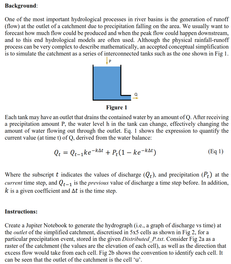
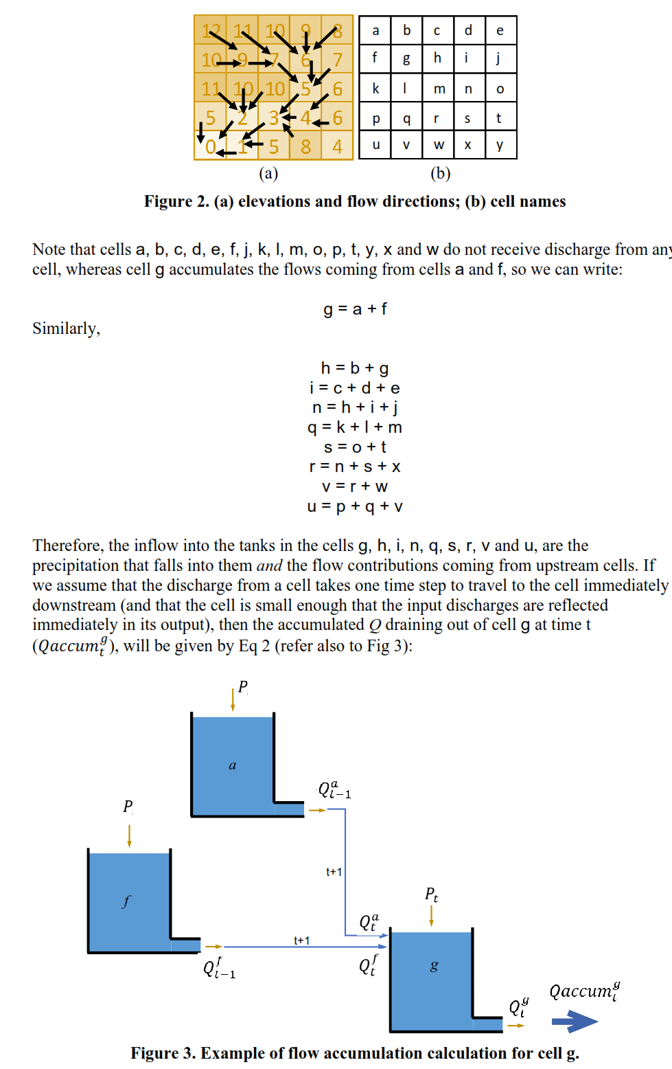
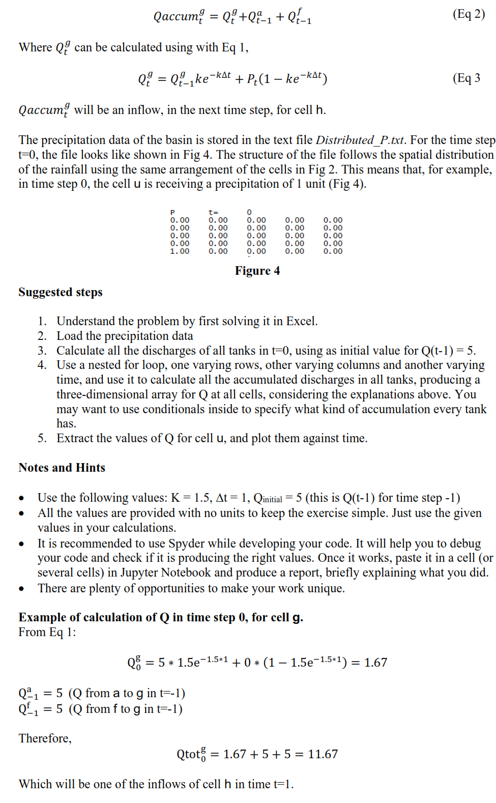
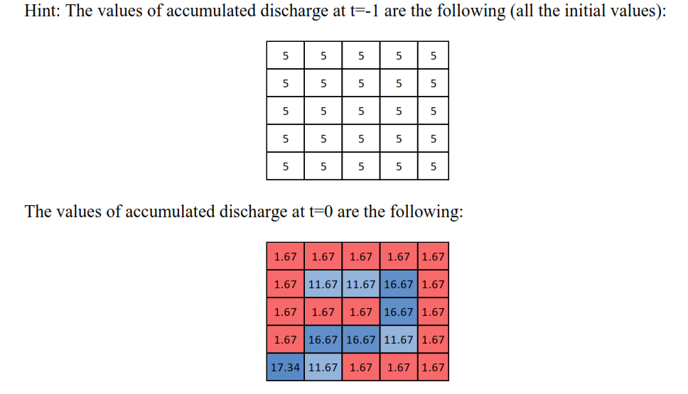
Background: One of the most important hydrological processes in river basins is the generation of runoff (flow) at the outlet of a catchment due to precipitation falling on the area. We usually want to forecast how much flow could be produced and when the peak flow could happen downstream, and to this end hydrological models are often used. Although the physical rainfall-runoff process can be very complex to describe mathematically, an accepted conceptual simplification is to simulate the catchment as a series of interconnected tanks such as the one shown in Fig 1. Q Figure 1 Each tank may have an outlet that drains the contained water by an amount of Q. After receiving a precipitation amount P, the water level h in the tank can change, effectively changing the amount of water flowing out through the outlet. Eq. 1 shows the expression to quantify the current value (at time t) of Q, derived from the water balance: Qt = - Qt-ke-kat +P+(1 ke-kat) (Eq 1) 1 Where the subscript t indicates the values of discharge (Qt), and precipitation (Pt) at the current time step, and Qt-1 is the previous value of discharge a time step before. In addition, k is a given coefficient and At is the time step. Instructions: Create a Jupiter Notebook to generate the hydrograph (i.e., a graph of discharge vs time) at the outlet of the simplified catchment, discretised in 5x5 cells as shown in Fig 2, for a particular precipitation event, stored in the given Distributed_P.txt. Consider Fig 2a as a raster of the catchment (the values are the elevation of each cell), as well as the direction that excess flow would take from each cell. Fig 2b shows the convention to identify each cell. It can be seen that the outlet of the catchment is the cell 'u'. a b d e f 09 i : f k p m m n 0 q a S t 10 h j 11 10,10526 1 3+4+ 5 8 (a) (b) Figure 2. (a) elevations and flow directions; (b) cell names u V w X Note that cells a, b, c, d, e, f, j, k, l, m, o, p, t, y, X and w do not receive discharge from any cell, whereas cell g accumulates the flows coming from cells a and f, so we can write: g= a +f Similarly, h = b + g i = c + d + e n= h + i + j q = k + + m S = o +t r= n + S + x v=r + w u= p + q + V Therefore, the inflow into the tanks in the cells g, h, i, n, q, s, r, V and u, are the precipitation that falls into them and the flow contributions coming from upstream cells. If we assume that the discharge from a cell takes one time step to travel to the cell immediately downstream (and that the cell is small enough that the input discharges are reflected immediately in its output), then the accumulated Q draining out of cell g at time t (Qaccum), will be given by Eq 2 (refer also to Fig 3): Qi-1 P t+1 Qa t+1 Q-1 e g Qaccum Qey Figure 3. Example of flow accumulation calculation for cell g. Qaccum = Q+Qx-1 +Q-1 = (Eq 2) -1 Where Qt can be calculated using with Eq 1, Q = Q!-ke -kt = + Pt(1 ke-kat) (Eq3 Qaccum, will be an inflow, in the next time step, for cell h. The precipitation data of the basin is stored in the text file Distributed_P.txt. For the time step t0, the file looks like shown in Fig 4. The structure of the file follows the spatial distribution of the rainfall using the same arrangement of the cells in Fig 2. This means that, for example, in time step 0, the cell u is receiving a precipitation of 1 unit (Fig 4). P 0.00 0.00 0.00 0.00 1.00 0.00 0.00 0.00 0.00 0.00 o 0.00 0.00 0.00 0.00 0.00 0.00 0.00 0.00 0.00 0.00 0.00 0.00 0.00 0.00 0.00 Figure 4 Suggested steps 1. Understand the problem by first solving it in Excel. 2. Load the precipitation data 3. Calculate all the discharges of all tanks in t=0, using as initial value for Q(t-1) = 5. 4. Use a nested for loop, one varying rows, other varying columns and another varying time, and use it to calculate all the accumulated discharges in all tanks, producing a three-dimensional array for Q at all cells, considering the explanations above. You may want to use conditionals inside to specify what kind of accumulation every tank has. 5. Extract the values of Q for cell u, and plot them against time. Notes and Hints . Use the following values: K= 1.5, At = 1, Qinitial = 5 (this is Q(t-1) for time step -1) All the values are provided with no units to keep the exercise simple. Just use the given values in your calculations. It is recommended to use Spyder while developing your code. It will help you to debug your code and check if it is producing the right values. Once it works, paste it in a cell (or several cells) in Jupyter Notebook and produce a report, briefly explaining what you did. There are plenty of opportunities to make your work unique. . Example of calculation of Q in time step 0, for cell g. From Eq 1: Q = 5 * 1.5e-1.5*1 +0* (1 1.5e-1.5*1) = = 1.67 Qa1 = 5 (Q from a to g in t=-1) Q-1 = 5 (Q from f to g in t=-1) Therefore, Qtot; = 1.67 +5+5 = 11.67 Which will be one of the inflows of cell h in time t=1. Hint: The values of accumulated discharge at t=-1 are the following (all the initial values): 5 5 5 5 5 5 5 5 5 5 5 5 5 5 5 5 5 5 5 5 5 5 5 5 5 The values of accumulated discharge at t=0 are the following: 1.67 1.67 1.67 1.67 1.67 1.67 11.67 11.67 16.67 1.67 1.67 1.67 1.67 16.67 1.67 1.67 16.67 16.67 11.67 1.67 17.34 11.67 1.67 1.67 1.67