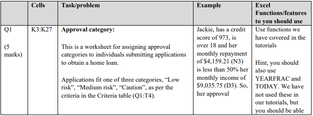
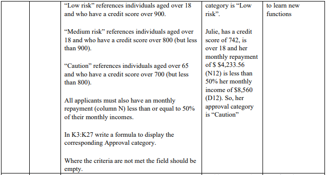
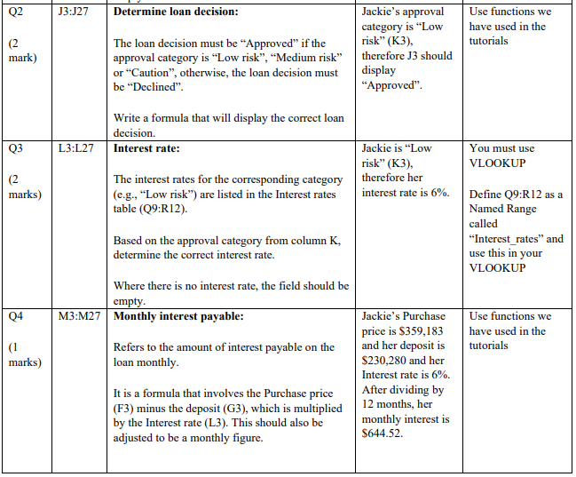
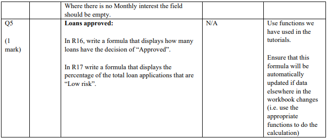
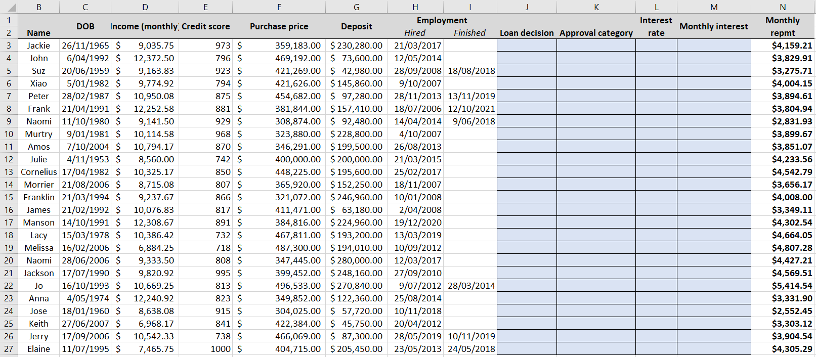
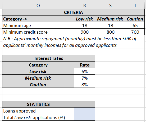
Q1 (5 marks) Cells Task/problem Example Excel Functions/features to you should use K3:K27 Approval category: Jackie, has a credit Use functions we score of 973, is have covered in the This is a worksheet for assigning approval over 18 and her tutorials categories to individuals submitting applications monthly repayment to obtain a home loan. of $4,159.21 (N3) Hint, you should is less than 50% her also use Applications fit one of three categories, Low monthly income of YEARFRAC and risk, Medium risk, Caution", as per the $9,035.75 (D3). So, TODAY. We have criteria in the Criteria table (Q1:14). her approval not used these in our tutorials, but you should be able Low risk references individuals aged over 18 and who have a credit score over 900. category is "Low risk" to learn new functions Medium risk" references individuals aged over Julie, has a credit 18 and who have a credit score over 800 (but less score of 742, is than 900). over 18 and her monthly repayment "Caution references individuals aged over 65 of $ $4,233.56 and who have a credit score over 700 (but less (N12) is less than than 800) 50% her monthly income of $8,560 All applicants must also have an monthly (D12). So, her repayment (column N) less than or equal to 50% approval category of their monthly incomes. is Caution" In K3:K27 write a formula to display the corresponding Approval category. Where the criteria are not met the field should be empty. Q2 J3:J27 Determine loan decision: Use functions we have used in the tutorials (2 mark) The loan decision must be Approved" if the approval category is "Low risk, Medium risk" or "Caution", otherwise, the loan decision must be Declined". Jackie's approval category is "Low risk" (K3), therefore J3 should display "Approved". Write a formula that will display the correct loan decision. Interest rate: Q3 L3:L27 Jackie is "Low risk (K3), therefore her interest rate is 6%. You must use VLOOKUP (2 marks) The interest rates for the corresponding category (e.g., "Low risk) are listed in the Interest rates table (Q9:R12). Based on the approval category from column K, determine the correct interest rate. Define 09:R12 as a Named Range called "Interest_rates" and use this in your VLOOKUP Where there is no interest rate, the field should be empty. M3:M27 Monthly interest payable: 04 Use functions we have used in the tutorials (1 Refers to the amount of interest payable on the loan monthly. marks) Jackie's Purchase price is $359,183 and her deposit is $230,280 and her Interest rate is 6%. After dividing by 12 months, her monthly interest is $644.52. It is a formula that involves the Purchase price (F3) minus the deposit (G3), which is multiplied by the Interest rate (L3). This should also be adjusted to be a monthly figure. Where there is no Monthly interest the field should be empty. Loans approved: Q5 N/A Use functions we have used in the tutorials. (1 mark) In R16, write a formula that displays how many loans have the decision of "Approved". In R17 write a formula that displays the percentage of the total loan applications that are "Low risk". Ensure that this formula will be automatically updated if data elsewhere in the workbook changes (i.e. use the appropriate functions to do the calculation) B D E M Interest Monthly interest rate 1 DOB Income (monthly Credit score 2. Name 3 Jackie 26/11/1965 $ 9,035.75 973 $ 4 John 6/04/1992 $ 12,372.50 796 $ 5 Suz 20/06/1959 $ 9,163.83 923 $ 6 Xiao 5/01/1982 $ 9,774.92 794 $ 7 Peter 28/02/1987 $ 10,950.08 875 $ 8 Frank 21/04/1991 $ 12,252.58 881 S 9 Naomi 11/10/1980 $ 9,141.50 929 $ 10 Murtry 9/01/1981 $ 10,114.58 968 $ 11 Amos 7/10/2004 $ 10,794.17 870 $ 12 Julie 4/11/1953 $ 8,560.00 742 $ 13 Cornelius 17/04/1982 $ 10,325.17 850 $ 14 Morrier 21/08/2006 $ 8,715.08 807 $ 15 Franklin 21/03/1994 $ 9,237.67 866 $ 16 James 21/02/1992 $ 10,076.83 817 S 17 Manson 14/10/1991 $ 12,308.67 891 $ 18 Lacy 15/03/1978 $ 10,386.42 732 $ 19 Melissa 16/02/2006 $ 6,884.25 718 $ 20 Naomi 28/06/2006 $ 9,333.50 808 $ 21 Jackson 17/07/1990 $ 9,820.92 995 $ 22 Jo 16/10/1993 $ 10,669.25 813 $ 23 Anna 4/05/1974 $ 12,240.92 823 $ 24 Jose 18/01/1960 $ 8,638.08 915 $ 25 Keith 27/06/2007 $ 6,968.17 841 $ 26 Jerry 17/09/2006 $ 10,542.33 738 $ 27 Elaine 11/07/1995 $ 7,465.75 1000 $ F G H K Purchase price Employment Deposit Hired Finished Loan decision Approval category 359,183.00 $ 230,280.00 21/03/2017 469,192.00 $ 73,600.00 12/05/2014 421,269.00 $ 42,980.00 28/09/2008 18/08/2018 421,626.00 $ 145,860.00 9/10/2007 454,682.00 $ 97,280.00 28/11/2013 13/11/2019 381,844.00 $ 157,410.00 18/07/2006 12/10/2021 308,874.00 $ 92,480.00 14/04/2014 9/06/2018 323,880.00 $ 228,800.00 4/10/2007 346,291.00 $ 199,500.00 26/08/2013 400,000.00 $ 200,000.00 21/03/2015 448,225.00 $ 195,600.00 25/02/2017 365,920.00 $ 152,250.00 18/11/2007 321,072.00 $ 246,960.00 10/01/2008 411,471.00 $ 63,180.00 2/04/2008 384,816.00 $ 224,960.00 19/12/2020 467,811.00 $ 193,200.00 13/03/2019 487,300.00 $ 194,010.00 10/09/2012 347,445.00 $ 280,000.00 12/03/2017 399,452.00 $ 248,160.00 27/09/2010 496,533.00 $ 270,840.00 9/07/2012 28/03/2014 349,852.00 $ 122,360.00 25/08/2014 304,025.00 $ 57,720.00 10/11/2018 422,384.00 $ 45,750.00 20/04/2012 466,069.00 $ 87,300.00 28/05/2019 10/11/2019 404,715.00 $ 205,450.00 23/05/2013 24/05/2018 N Monthly repmt $4,159.21 $3,829.91 $3,275.71 $4,004.15 $3,894.61 $3,804.94 $2,831.93 $3,899.67 $3,851.07 $4,233.56 $4,542.79 $3,656.17 $4,008.00 $3,349.11 $4,302.54 $4,664.05 $4,807.28 $4,427.21 $4,569.51 $5,414.54 $3,331.90 $2,552.45 $3,303.12 $3,904.54 $4,305.29 Q R S CRITERIA Category -> Low risk Medium risk Caution Minimum age 18 18 65 Minimum credit score 900 800 700 N.B.: Approximate repayment (monthly) must be less than 50% of applicants' monthly incomes for all approved applicants Rate Interest rates Category Low risk Medium risk Caution 6% 7% 8% STATISTICS Loans approved Total Low risk applications (%) Q1 (5 marks) Cells Task/problem Example Excel Functions/features to you should use K3:K27 Approval category: Jackie, has a credit Use functions we score of 973, is have covered in the This is a worksheet for assigning approval over 18 and her tutorials categories to individuals submitting applications monthly repayment to obtain a home loan. of $4,159.21 (N3) Hint, you should is less than 50% her also use Applications fit one of three categories, Low monthly income of YEARFRAC and risk, Medium risk, Caution", as per the $9,035.75 (D3). So, TODAY. We have criteria in the Criteria table (Q1:14). her approval not used these in our tutorials, but you should be able Low risk references individuals aged over 18 and who have a credit score over 900. category is "Low risk" to learn new functions Medium risk" references individuals aged over Julie, has a credit 18 and who have a credit score over 800 (but less score of 742, is than 900). over 18 and her monthly repayment "Caution references individuals aged over 65 of $ $4,233.56 and who have a credit score over 700 (but less (N12) is less than than 800) 50% her monthly income of $8,560 All applicants must also have an monthly (D12). So, her repayment (column N) less than or equal to 50% approval category of their monthly incomes. is Caution" In K3:K27 write a formula to display the corresponding Approval category. Where the criteria are not met the field should be empty. Q2 J3:J27 Determine loan decision: Use functions we have used in the tutorials (2 mark) The loan decision must be Approved" if the approval category is "Low risk, Medium risk" or "Caution", otherwise, the loan decision must be Declined". Jackie's approval category is "Low risk" (K3), therefore J3 should display "Approved". Write a formula that will display the correct loan decision. Interest rate: Q3 L3:L27 Jackie is "Low risk (K3), therefore her interest rate is 6%. You must use VLOOKUP (2 marks) The interest rates for the corresponding category (e.g., "Low risk) are listed in the Interest rates table (Q9:R12). Based on the approval category from column K, determine the correct interest rate. Define 09:R12 as a Named Range called "Interest_rates" and use this in your VLOOKUP Where there is no interest rate, the field should be empty. M3:M27 Monthly interest payable: 04 Use functions we have used in the tutorials (1 Refers to the amount of interest payable on the loan monthly. marks) Jackie's Purchase price is $359,183 and her deposit is $230,280 and her Interest rate is 6%. After dividing by 12 months, her monthly interest is $644.52. It is a formula that involves the Purchase price (F3) minus the deposit (G3), which is multiplied by the Interest rate (L3). This should also be adjusted to be a monthly figure. Where there is no Monthly interest the field should be empty. Loans approved: Q5 N/A Use functions we have used in the tutorials. (1 mark) In R16, write a formula that displays how many loans have the decision of "Approved". In R17 write a formula that displays the percentage of the total loan applications that are "Low risk". Ensure that this formula will be automatically updated if data elsewhere in the workbook changes (i.e. use the appropriate functions to do the calculation) B D E M Interest Monthly interest rate 1 DOB Income (monthly Credit score 2. Name 3 Jackie 26/11/1965 $ 9,035.75 973 $ 4 John 6/04/1992 $ 12,372.50 796 $ 5 Suz 20/06/1959 $ 9,163.83 923 $ 6 Xiao 5/01/1982 $ 9,774.92 794 $ 7 Peter 28/02/1987 $ 10,950.08 875 $ 8 Frank 21/04/1991 $ 12,252.58 881 S 9 Naomi 11/10/1980 $ 9,141.50 929 $ 10 Murtry 9/01/1981 $ 10,114.58 968 $ 11 Amos 7/10/2004 $ 10,794.17 870 $ 12 Julie 4/11/1953 $ 8,560.00 742 $ 13 Cornelius 17/04/1982 $ 10,325.17 850 $ 14 Morrier 21/08/2006 $ 8,715.08 807 $ 15 Franklin 21/03/1994 $ 9,237.67 866 $ 16 James 21/02/1992 $ 10,076.83 817 S 17 Manson 14/10/1991 $ 12,308.67 891 $ 18 Lacy 15/03/1978 $ 10,386.42 732 $ 19 Melissa 16/02/2006 $ 6,884.25 718 $ 20 Naomi 28/06/2006 $ 9,333.50 808 $ 21 Jackson 17/07/1990 $ 9,820.92 995 $ 22 Jo 16/10/1993 $ 10,669.25 813 $ 23 Anna 4/05/1974 $ 12,240.92 823 $ 24 Jose 18/01/1960 $ 8,638.08 915 $ 25 Keith 27/06/2007 $ 6,968.17 841 $ 26 Jerry 17/09/2006 $ 10,542.33 738 $ 27 Elaine 11/07/1995 $ 7,465.75 1000 $ F G H K Purchase price Employment Deposit Hired Finished Loan decision Approval category 359,183.00 $ 230,280.00 21/03/2017 469,192.00 $ 73,600.00 12/05/2014 421,269.00 $ 42,980.00 28/09/2008 18/08/2018 421,626.00 $ 145,860.00 9/10/2007 454,682.00 $ 97,280.00 28/11/2013 13/11/2019 381,844.00 $ 157,410.00 18/07/2006 12/10/2021 308,874.00 $ 92,480.00 14/04/2014 9/06/2018 323,880.00 $ 228,800.00 4/10/2007 346,291.00 $ 199,500.00 26/08/2013 400,000.00 $ 200,000.00 21/03/2015 448,225.00 $ 195,600.00 25/02/2017 365,920.00 $ 152,250.00 18/11/2007 321,072.00 $ 246,960.00 10/01/2008 411,471.00 $ 63,180.00 2/04/2008 384,816.00 $ 224,960.00 19/12/2020 467,811.00 $ 193,200.00 13/03/2019 487,300.00 $ 194,010.00 10/09/2012 347,445.00 $ 280,000.00 12/03/2017 399,452.00 $ 248,160.00 27/09/2010 496,533.00 $ 270,840.00 9/07/2012 28/03/2014 349,852.00 $ 122,360.00 25/08/2014 304,025.00 $ 57,720.00 10/11/2018 422,384.00 $ 45,750.00 20/04/2012 466,069.00 $ 87,300.00 28/05/2019 10/11/2019 404,715.00 $ 205,450.00 23/05/2013 24/05/2018 N Monthly repmt $4,159.21 $3,829.91 $3,275.71 $4,004.15 $3,894.61 $3,804.94 $2,831.93 $3,899.67 $3,851.07 $4,233.56 $4,542.79 $3,656.17 $4,008.00 $3,349.11 $4,302.54 $4,664.05 $4,807.28 $4,427.21 $4,569.51 $5,414.54 $3,331.90 $2,552.45 $3,303.12 $3,904.54 $4,305.29 Q R S CRITERIA Category -> Low risk Medium risk Caution Minimum age 18 18 65 Minimum credit score 900 800 700 N.B.: Approximate repayment (monthly) must be less than 50% of applicants' monthly incomes for all approved applicants Rate Interest rates Category Low risk Medium risk Caution 6% 7% 8% STATISTICS Loans approved Total Low risk applications (%)