Q.5
(question 3,4 are completed)
NEXT, Perform a statistical residual analysis of the relationship to remove outliers. Report on the revised regression without these outliers, in terms of effect size and F test format Also explain how ERIratio predicted sIgA better, or worse, without these outliers.This is excel link for syntax question 5 :)
SYNTAX
https://docs.google.com/document/d/1ZzY4AEoby8NCsPwmP96aLnv7FehHc2TwELyaFmyv_WE/edit?usp=sharing
EXCEL DATA
https://docs.google.com/spreadsheets/d/1a6FiZmx2WWqDSqRV3E5SLORHRMi3fr3vHQTJwg2yrds/edit?usp=sharing
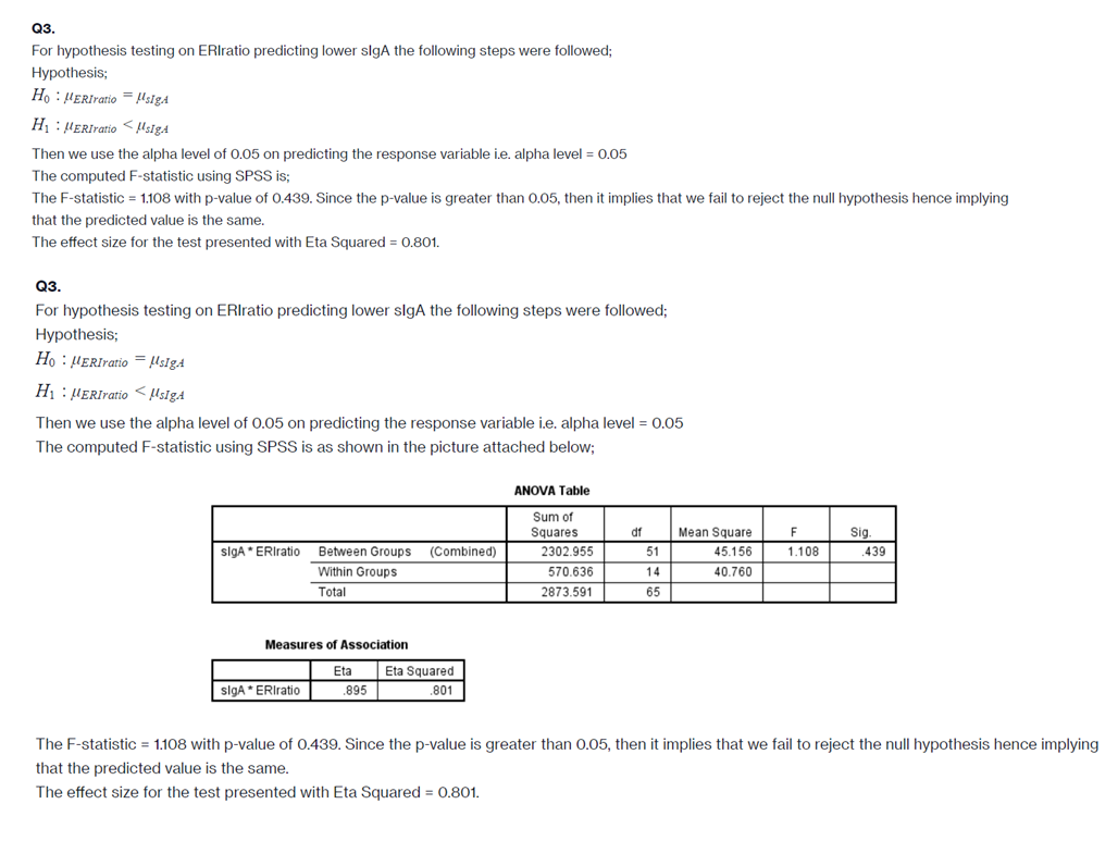
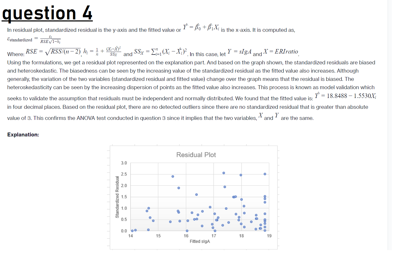
Q3. For hypothesis testing on ERIratio predicting lower sigA the following steps were followed; Hypothesis; Ho : MERIratio = UsigA H1 : MERIratio Msign Then we use the alpha level of 0.05 on predicting the response variable i.e. alpha level = 0.05 The computed F-statistic using SPSS is; The F-statistic = 1.108 with p-value of 0.439. Since the p-value is greater than 0.05, then it implies that we fail to reject the null hypothesis hence implying that the predicted value is the same. The effect size for the test presented with Eta Squared = 0.801. Q3. For hypothesis testing on ERIratio predicting lower sigA the following steps were followed; Hypothesis; Ho : HERIratio = MsigA H1 : MERIratio MsigA Then we use the alpha level of 0.05 on predicting the response variable i.e. alpha level = 0.05 The computed F-statistic using SPSS is as shown in the picture attached below; ANOVA Table Sum of Squares Mean Square Sig sigA * ERiratio Between Groups (Combined) 2302.955 51 45.156 1.108 439 Within Groups 570.636 14 40.760 Total 2873.591 65 Measures of Association Eta Eta Squared sigA * ERIratio 895 801 The F-statistic = 1.108 with p-value of 0.439. Since the p-value is greater than 0.05, then it implies that we fail to reject the null hypothesis hence implying that the predicted value is the same. The effect size for the test presented with Eta Squared = 0.801.question 4 In residual plot, standardized residual is the ysaxis and the fitted value or F = 3}) +'1Xi is the xsaxis. It is computed as, . = 5i Ss'randaldlzed R SE 1F}?! 7 _ 1 (XJ'EA 7 n 7 7 . Where: RSE T V RSS/(rr 2), hi H + SSX and SSX Zi=1(Xl 02. In this case, let Y TSIgA and X7 ERIratro Using the formulations, we get a residual plot represented on the explanation part. And based on the graph shown, the standardized residuals are biased and heteroskedastic. The biasedness can be seen by the increasing value of the standardized residual as the fitted value also increases. Although generally, the variation of the two variables (standardized residual and fitted value) change over the graph means that the residual is biased. The heteroskedasticity can be seen by the increasing dispersion of points as the fitted value also increases. This process is known as model validation which #2 18.8488 71.5530Xi seeks to validate the assumption that residuals must be independent and normally distributed. We found that the fitted value is: in four decimal places. Based on the residual plot, there are no detected outliers since there are no standardized residual that is greater than absolute X value of 3. This confirms the ANOVA test conducted in question 3 since it implies that the two variables, and Y are the same. Explanation: Residual Plot 3.0 a 25 . ' o 0 3 2.11 . . O E 15 " . I g 0 U 10 . ' o ' g ' 0 . ' o o. 0 . o 05 . . . . o- ..f. . u. .o.! O 0.0 a. 0 o .0 . ": 14 15 16 17 1a 19 Filled SlgA


