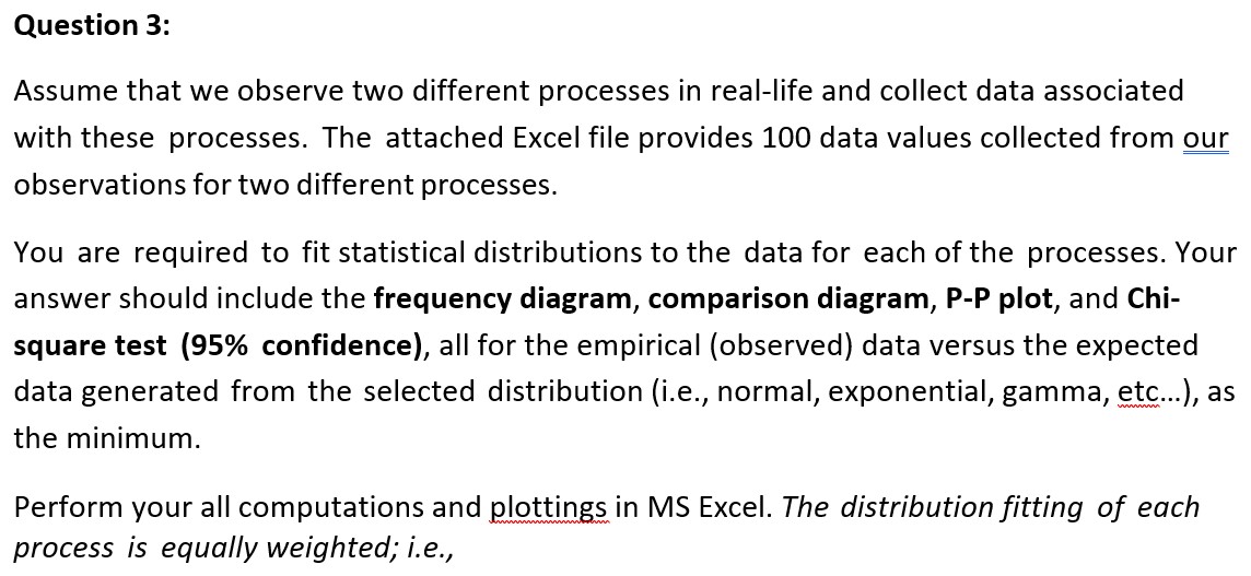
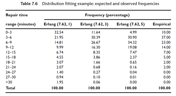
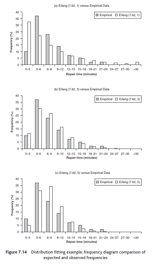
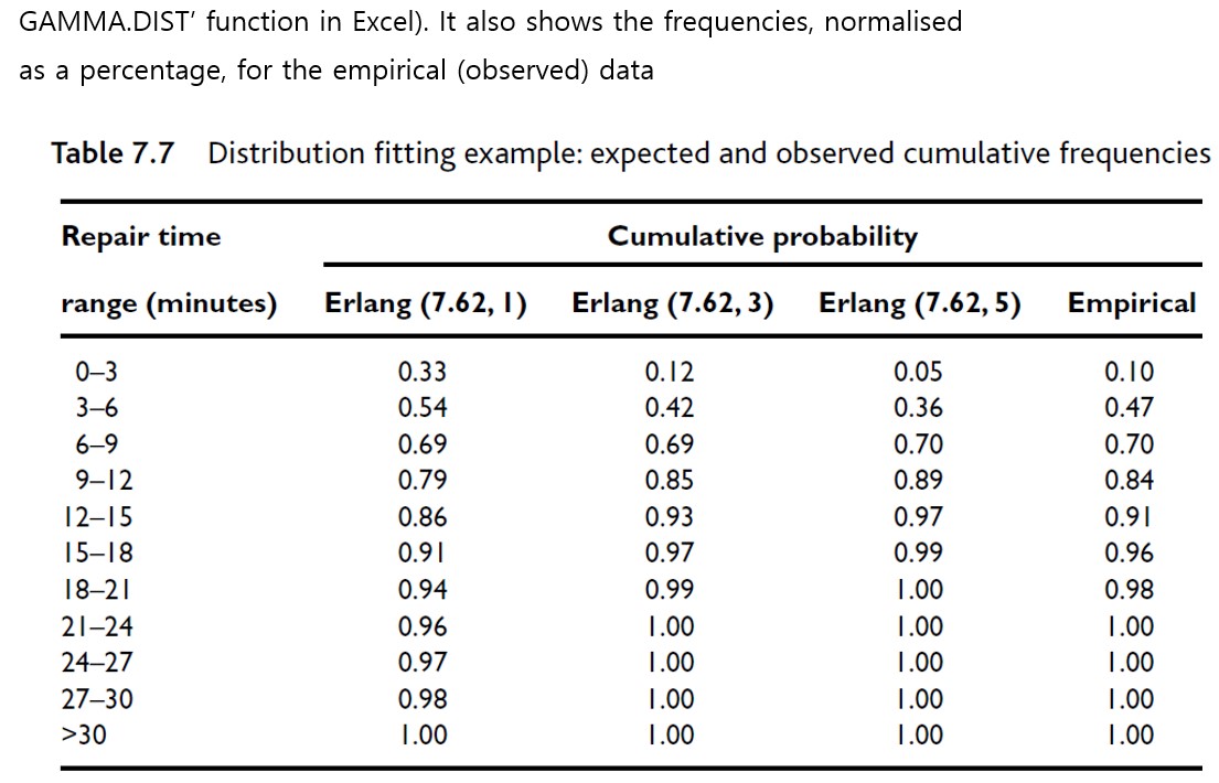
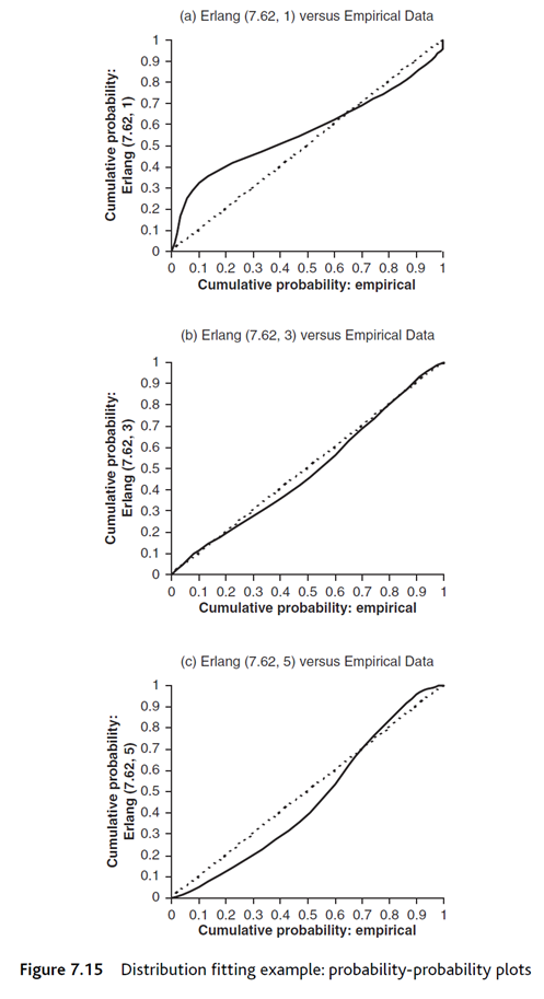
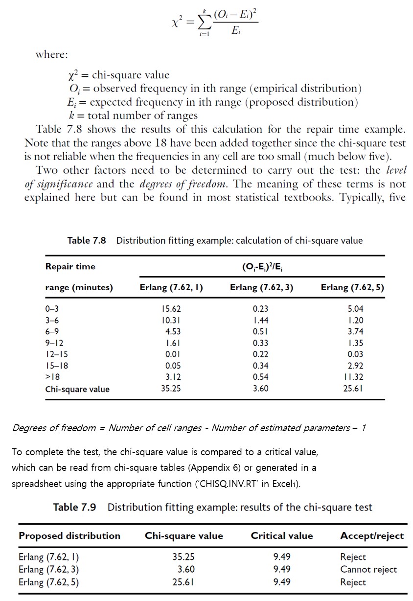
Question 3: Assume that we observe two different processes in real-life and collect data associated with these processes. The attached Excel file provides 100 data values collected from our observations for two different processes. You are required to fit statistical distributions to the data for each of the processes. Your answer should include the frequency diagram, comparison diagram, P-P plot, and Chi- square test (95% confidence), all for the empirical (observed) data versus the expected data generated from the selected distribution (i.e., normal, exponential, gamma, etc...), as the minimum. Perform your all computations and plottings in MS Excel. The distribution fitting of each process is equally weighted; i.e., Table 7.6 Distribution fitting example: expected and observed frequencies Repair time Frequency (percentage) range (minutes) Erlang (7.62, 1) Erlang (7.62,3) Erlang (7.62,5) Empirical 0-3 32.54 11.64 4.99 10.00 3-6 6-9 21.95 30.39 30.90 37.00 14.81 26.67 34.32 23.00 9-12 9.99 16.30 19.08 14.00 12-15 6.74 8.35 7.47 7.00 15-18 4.55 3.86 2.37 5.00 18-21 3.07 1.66 0.65 2.00 21-24 2.07 0.68 0.16 2.00 24-27 1.40 0.27 0.04 0.00 27-30 0.94 0.10 0.01 0.00 >30 1.95 0.06 0.00 0.00 Total 100.00 100.00 100.00 100.00 40 35 30 25 20 2250 10 Frequency (%) 50 (a) Erlang (7.62, 1) versus Empirical Data Empirical Erlang (7.62, 1) 0+ 0-3 3-6 6-9 9-12 12-15 15-18 18-21 21-24 24-27 27-30 >30 Repair time (minutes) Empirical Erlang (7.62, 3) 40 (b) Erlang (7.62, 3) versus Empirical Data 35 30- 25 20 15 2 3 3 2 2 50 10 Frequency (%) 50 0-3 Frequency (%) 20 15 NNW & 30 25 40 35 3-6 6-9 9-12 12-15 15-18 18-21 21-24 24-27 27-30 Repair time (minutes) >30 10 5 0-3 3-6 (c) Erlang (7.62, 5) versus Empirical Data Empirical Erlang (7.62, 5) 6-9 9-12 12-15 15-18 18-21 21-24 24-27 27-30 >30 Repair time (minutes) Figure 7.14 Distribution fitting example: frequency diagram comparison of expected and observed frequencies GAMMA.DIST' function in Excel). It also shows the frequencies, normalised as a percentage, for the empirical (observed) data Table 7.7 Distribution fitting example: expected and observed cumulative frequencies Repair time Cumulative probability range (minutes) Erlang (7.62, 1) Erlang (7.62, 3) Erlang (7.62, 5) Empirical 0-3 0.33 0.12 0.05 0.10 3-6 0.54 0.42 0.36 0.47 6-9 0.69 0.69 0.70 0.70 9-12 0.79 0.85 0.89 0.84 12-15 0.86 0.93 0.97 0.91 15-18 0.91 0.97 0.99 0.96 18-21 0.94 0.99 1.00 0.98 21-24 0.96 1.00 1.00 1.00 24-27 0.97 1.00 1.00 1.00 27-30 0.98 1.00 1.00 1.00 >30 1.00 1.00 1.00 1.00 Cumulative probability: Erlang (7.62, 1) Cumulative probability: Erlang (7.62, 3) Cumulative probability: Erlang (7.62, 5) 1 0.9 0.8 65 0.6 0.5 0.4 0.3 0.2 0.1 0 0.9 0.8 7654 3 2 0.5 0.4 0.3 (a) Erlang (7.62, 1) versus Empirical Data 0 0.1 0.2 0.3 0.4 0.5 0.6 0.7 0.8 0.9 1 Cumulative probability: empirical (b) Erlang (7.62, 3) versus Empirical Data 0.2- 0.1 0 0 0.1 0.2 0.3 0.4 0.5 0.6 0.7 0.8 0.9 1 Cumulative probability: empirical 0.9 0.8 0.6 0.5 0.4 0.3 0.2 (c) Erlang (7.62, 5) versus Empirical Data 0.1 0 0 0.1 0.2 0.3 0.4 0.5 0.6 0.7 0.8 0.9 1 Cumulative probability: empirical Figure 7.15 Distribution fitting example: probability-probability plots Ei i=1 where: x2 chi-square value = O; observed frequency in ith range (empirical distribution) E;= expected frequency in ith range (proposed distribution) k = total number of ranges Table 7.8 shows the results of this calculation for the repair time example. Note that the ranges above 18 have been added together since the chi-square test is not reliable when the frequencies in any cell are too small (much below five). Two other factors need to be determined to carry out the test: the level of significance and the degrees of freedom. The meaning of these terms is not explained here but can be found in most statistical textbooks. Typically, five Table 7.8 Distribution fitting example: calculation of chi-square value Repair time range (minutes) (O-E)/E Erlang (7.62, 1) Erlang (7.62, 3) Erlang (7.62,5) 0-3 15.62 0.23 5.04 3-6 10.31 1.44 1.20 6-9 4.53 0.51 3.74 9-12 1.61 0.33 1.35 12-15 0.01 0.22 0.03 15-18 0.05 0.34 2.92 >18 3.12 0.54 11.32 Chi-square value 35.25 3.60 25.61 Degrees of freedom = Number of cell ranges - Number of estimated parameters - 1 To complete the test, the chi-square value is compared to a critical value, which can be read from chi-square tables (Appendix 6) or generated in a spreadsheet using the appropriate function ('CHISQ. INV.RT' in Excel1). Table 7.9 Distribution fitting example: results of the chi-square test Proposed distribution Chi-square value Critical value Accept/reject Erlang (7.62, 1) 35.25 9.49 Reject Erlang (7.62, 3) 3.60 9.49 Cannot reject Erlang (7.62, 5) 25.61 9.49 Reject