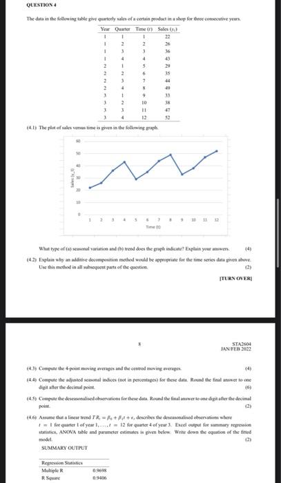
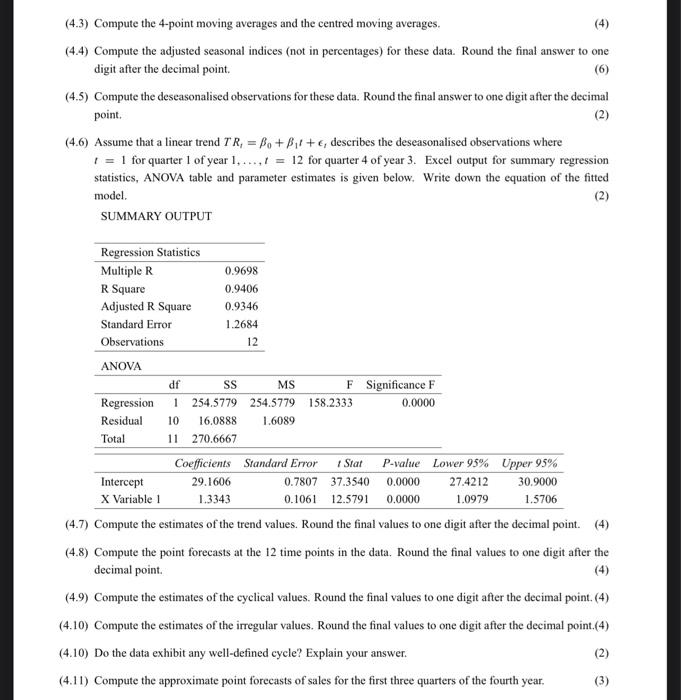
QUESTION 4 The data in the following table give quarterly sales of a certain product in a shop for there comective years Year Quarter Time Sales 1 1 1 1 2 2 26 1 3 3 36 1 4 4 1 5 29 2 6 35 7 44 4 * 9 33 10 47 4 12 52 (4.) The plot of sales venus time is given in the following up 65 What type of seasonal variation and by trend does the graph indicate! Explain your own (4) (42) Explain why an additive decomposition method would be appropriate for the time series duta given above Use this method in all boot parts of the question C) TURN OVERI STA2604 JAN FER 2022 (4) (43) Compute the pemeving wage and the centred mering av (44) Compute the adjusted sconal indices (not in percentages for these date Round the final anwer to che digit after the decimal point 16) (49) Compute the disease observations for these data Round the finalmente ne digitalter the decimal 6. Assume that a linear Tron TR = R + Bil + describes the descanalised obicnations where + 1 for quarter of year... 12 fe quarter of your 3. Excel output for summary represim statistics, ANOVA ble and parameter estimates is given below Write down the equation of the fined SUMMARY OUTPUT Regression Statistics Multiple 0.99 0.90 RS (4.3) Compute the 4-point moving averages and the centred moving averages. (4) (4.4) Compute the adjusted seasonal indices (not in percentages) for these data. Round the final answer to one digit after the decimal point (6) (4.5) Compute the deseasonalised observations for these data. Round the final answer to one digit after the decimal point. (2) (4.6) Assume that a linear trend TR, = Bo + Bit + e, describes the deseasonalised observations where 1 = 1 for quarter 1 of year 1.....I = 12 for quarter 4 of year 3. Excel output for summary regression statistics, ANOVA table and parameter estimates is given below. Write down the equation of the fitted model. (2) SUMMARY OUTPUT Regression Statistics Multiple R 0.9698 R Square 0.9406 Adjusted R Square 0.9346 Standard Error 1.2684 Observations 12 ANOVA df SS MS F Significance F Regression 1 254.5779 254.5779 158.2333 0.0000 Residual 10 16.0888 1.6089 Total 11 270.6667 Coefficients Standard Error 1 Stat P-value Lower 95% Upper 95% Intercept 29.1606 0.7807 37.3540 0.0000 27.4212 30.9000 X Variable 1 1.3343 0.1061 12.5791 0.0000 1.0979 1.5706 (4.7) Compute the estimates of the trend values. Round the final values to one digit after the decimal point. (4) (4.8) Compute the point forecasts at the 12 time points in the data. Round the final values to one digit after the decimal point (4.9) Compute the estimates of the cyclical values. Round the final values to one digit after the decimal point. (4) (4.10) Compute the estimates of the irregular values. Round the final values to one digit after the decimal point.(4) (4.10) Do the data exhibit any well-defined cycle? Explain your answer. (2) (4.11) Compute the approximate point forecasts of sales for the first three quarters of the fourth year. (3) QUESTION 4 The data in the following table give quarterly sales of a certain product in a shop for there comective years Year Quarter Time Sales 1 1 1 1 2 2 26 1 3 3 36 1 4 4 1 5 29 2 6 35 7 44 4 * 9 33 10 47 4 12 52 (4.) The plot of sales venus time is given in the following up 65 What type of seasonal variation and by trend does the graph indicate! Explain your own (4) (42) Explain why an additive decomposition method would be appropriate for the time series duta given above Use this method in all boot parts of the question C) TURN OVERI STA2604 JAN FER 2022 (4) (43) Compute the pemeving wage and the centred mering av (44) Compute the adjusted sconal indices (not in percentages for these date Round the final anwer to che digit after the decimal point 16) (49) Compute the disease observations for these data Round the finalmente ne digitalter the decimal 6. Assume that a linear Tron TR = R + Bil + describes the descanalised obicnations where + 1 for quarter of year... 12 fe quarter of your 3. Excel output for summary represim statistics, ANOVA ble and parameter estimates is given below Write down the equation of the fined SUMMARY OUTPUT Regression Statistics Multiple 0.99 0.90 RS (4.3) Compute the 4-point moving averages and the centred moving averages. (4) (4.4) Compute the adjusted seasonal indices (not in percentages) for these data. Round the final answer to one digit after the decimal point (6) (4.5) Compute the deseasonalised observations for these data. Round the final answer to one digit after the decimal point. (2) (4.6) Assume that a linear trend TR, = Bo + Bit + e, describes the deseasonalised observations where 1 = 1 for quarter 1 of year 1.....I = 12 for quarter 4 of year 3. Excel output for summary regression statistics, ANOVA table and parameter estimates is given below. Write down the equation of the fitted model. (2) SUMMARY OUTPUT Regression Statistics Multiple R 0.9698 R Square 0.9406 Adjusted R Square 0.9346 Standard Error 1.2684 Observations 12 ANOVA df SS MS F Significance F Regression 1 254.5779 254.5779 158.2333 0.0000 Residual 10 16.0888 1.6089 Total 11 270.6667 Coefficients Standard Error 1 Stat P-value Lower 95% Upper 95% Intercept 29.1606 0.7807 37.3540 0.0000 27.4212 30.9000 X Variable 1 1.3343 0.1061 12.5791 0.0000 1.0979 1.5706 (4.7) Compute the estimates of the trend values. Round the final values to one digit after the decimal point. (4) (4.8) Compute the point forecasts at the 12 time points in the data. Round the final values to one digit after the decimal point (4.9) Compute the estimates of the cyclical values. Round the final values to one digit after the decimal point. (4) (4.10) Compute the estimates of the irregular values. Round the final values to one digit after the decimal point.(4) (4.10) Do the data exhibit any well-defined cycle? Explain your answer. (2) (4.11) Compute the approximate point forecasts of sales for the first three quarters of the fourth year. (3)


