

Question:
Assignment #3: Independent Samples T test
Conduct an Independent Samples T test to answer the questions based on the following scenario. (Assume a nondirectional research hypothesis (two tailed test) and a level of significance of .05)
The superintendent who collected data for Assignments 1 and 2, continued to examine the district's data. One question that concerned the superintendent's constituencies was the difference between the school performance scores of the superintendent's district and a neighboring district that had similar demographic and socio-economic characteristics. The superintendent collected the following information:
School performance scores for superintendent's district:
109 108 133 146 120 84 102 124 148 155 87 144 158 159 126 80 118 130 83 129
153 137 136 96 138 110 156 99 152 113 143 128 103 161 123 89 82 140 112 154
School performance scores for comparison district:
140 154 115 152 104 111 148 91 88 130 114 100 117 95 109 120 103 146 93
134 132 112 122 147 151 137 84 149 85 156 128 157 96 127
What are the mean and standard deviation for the superintendent's district?
What are the mean and standard deviation for the comparison district?
State an appropriate null hypothesis for this analysis.
What is the observed or computed value of t?
What is the value of the degrees of freedom that are reported in the output (equal variances assumed)?
What is the reported level of significance?
Based on the reported level of significance, would you reject the null hypothesis?
Present the results as they might appear in an article. This must include a table and narrative statement that reports and interprets the results of the Independent Samples T test.
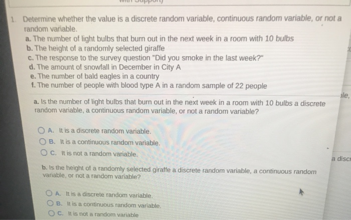
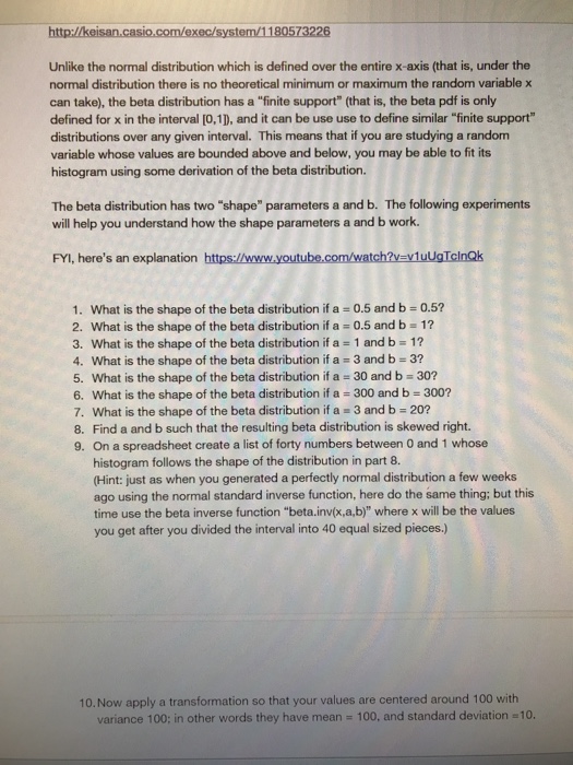
The Spectral Method in NWP: The spectral method in NWP is described by illustrating the spectral theory in general terms, as well as by applying this theory to the implementation of a specific spectral NWP model. The description of the implementation of this model, named PEAK, so as to illuminate all the building blocks that constitute a spectral global NWP model. PEAK is using this numerical method for the discretization of the continuous model equations in the horizontal directions. The spectral method is nowadays widely used in the formulation of global numerical weather prediction (NWP) models that simulate and predict the weather phenomena occurring in the Earth's atmosphere. The popularity of the spectral method relates to the fact that it naturally accounts for the spherical geometry of the Earth. Further, the spectral method is highly competitive in terms of its accuracy when compared to a grid-point method. The transform method has, in conjunction with the fast Fourier transform (FFT), provided for fundamentally reducing the computational complexity of the spectral method. Thus, having been considered a tool for a few low dimensional theoretical problems before 1970, the advent of the transform method has turned the spectral method into the most widely used numerical method in global NWP modeling. The numerical approach of the spectral method is used in the design of PEAK as an efficient, accurate, and standard tool widely used in global weather and climate modeling. The spectral method, in conjunction with the transform method, an energy-conserving vertical-differencing approach, and semi-implicit time differenceng provide the basic ingredients in the model construction.5. (a) State the Spectral Theorem for Symmetric matrices. (b) Write out the spectral factorization of 5 2 A = 2 2 (c) Using the change of variables x = Qy, where Q is an appropriate orthogonal matric, express the quadratic form 5r, + 4r142 + 21% in terms of y and y2. Describe and sketch the graph of the equation 5r, + 4712 + 2x2 = 1 in the T1, 12 plane. (d) Find the spectral decomposition of A.1. Determine whether the value is a discrete random variable, continuous random variable, or not a random variable. a. The number of light bulbs that burn out in the next week in a room with 10 bulbs b. The height of a randomly selected giraffe c. The response to the survey question "Did you smoke in the last week?" d. The amount of snowfall in December in City A e. The number of bald eagles in a country f. The number of people with blood type A in a random sample of 22 people ile, a. Is the number of light bulbs that burn out in the next week in a room with 10 bulbs a discrete random variable, a continuous random variable, or not a random variable? O A. It is a discrete random variable. O B. It is a continuous random variable. O C. It is not a random variable. a disc b. Is the height of a randomly selected giraffe a discrete random variable, a continuous random variable, or not a random variable? O A. It is a discrete random variable. O B. It is a continuous random variable. O C. It is not a random variablehttp://keisan.casio.com/exec/system/1180573226 Unlike the normal distribution which is defined over the entire x-axis (that is, under the normal distribution there is no theoretical minimum or maximum the random variable x can take), the beta distribution has a "finite support" (that is, the beta pdf is only defined for x in the interval [0,1]), and it can be use use to define similar "finite support" distributions over any given interval. This means that if you are studying a random variable whose values are bounded above and below, you may be able to fit its histogram using some derivation of the beta distribution. The beta distribution has two "shape" parameters a and b. The following experiments will help you understand how the shape parameters a and b work. FYI, here's an explanation https://www.youtube.com/watch?v=v1uUgTelnQk 1. What is the shape of the beta distribution if a = 0.5 and b = 0.5? 2. What is the shape of the beta distribution if a = 0.5 and b = 1? 3. What is the shape of the beta distribution if a = 1 and b = 1? 4. What is the shape of the beta distribution if a = 3 and b = 3? 5. What is the shape of the beta distribution if a = 30 and b = 30? 6. What is the shape of the beta distribution if a = 300 and b = 300? 7. What is the shape of the beta distribution if a = 3 and b = 20? 8. Find a and b such that the resulting beta distribution is skewed right. 9. On a spreadsheet create a list of forty numbers between 0 and 1 whose histogram follows the shape of the distribution in part 8. (Hint: just as when you generated a perfectly normal distribution a few weeks ago using the normal standard inverse function, here do the same thing; but this time use the beta inverse function "beta.inv(x,a,b)" where x will be the values you get after you divided the interval into 40 equal sized pieces.) 10. Now apply a transformation so that your values are centered around 100 with variance 100; in other words they have mean = 100, and standard deviation =10


