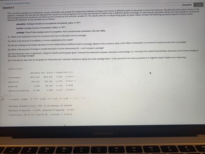
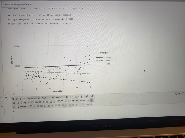
Question Completion Status: Question 4 54 points This is another question on moderation. As you remember, we studied the relationship between prestige and income at different levels of education in one of our lectures. We will look at the same results in this question. However this time we will interpret the results from the perspective of income and education relationship at different levels of prestige. In other words, education will be our main predictor variable and prestige will be the moderator (Z) while income remains as the outcome variable (V). The results with the corresponding graph are given below. Answer the following questions based on those results. Operational definition of the variables are as follows: education: Average education of occupational incumbent years, in 1971 income: Average income of incumbentis, dollars, in 1971 prestige: Pineo-Porter prestige score for occupation, from a social survey conducted in the mid-1960 Q1. What is the predicted income for someone who has no education and no prestige? 02. What is the amount of variability in income explained by the model Q3. We are looking at the simple education-income relationship at different levels of prestige. Based on this scenario what is the effect of education on income for someone who has no prestige? Q4. What is the amount of change in simple education-income relationship for 1 unit increase in prestige? 5. The interaction term is significant. Using the results and the graph given, interpret the interaction between education and prestige, le, how does the relationship between education and income change as the value of prestige changes. 06. If we were to add a line to the graph for those who are 2 standard deviations above the mean prestige level (+250)would the line have a positive or a negative slope? Explain your reasoning Coefficients Intercepti education Estimate Std. Error t value Petit B076.663 3903.035 0.0412 -993.023 402.441 -2.472 0.0151 - 86.453 0.102 0.9108 16.582 6.989 2.323 0.0196 prestige education prestige ---Signif. code: ***** 0.001 **** 0.01 **+ 0.05. 0.1.1 Residual standard error: 2921 on 90 degrees of freedom Yaltiple R-squared: 0.5408, Adjusted R-squared: 0.5267 Y-statistici 38.47 en 3 and 98 DF, p-value: