Question: Question: Simulink model: We have been designing our controllers with dynamics elements, including filters, integrators, and derivatives. In our analysis, we represent these using Laplace
Question:

 Simulink model:

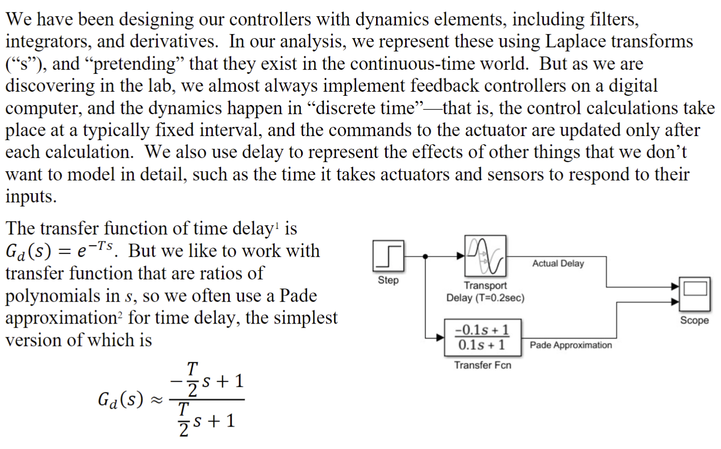
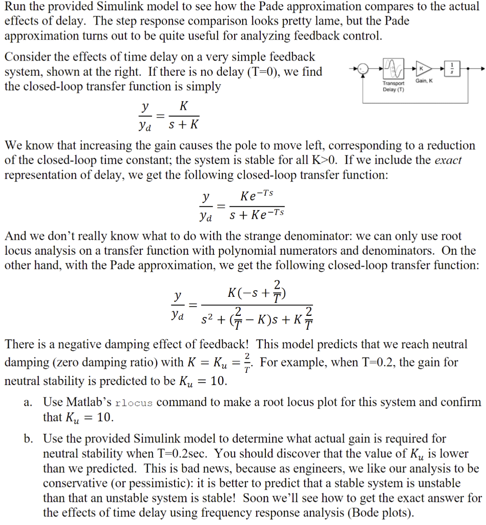
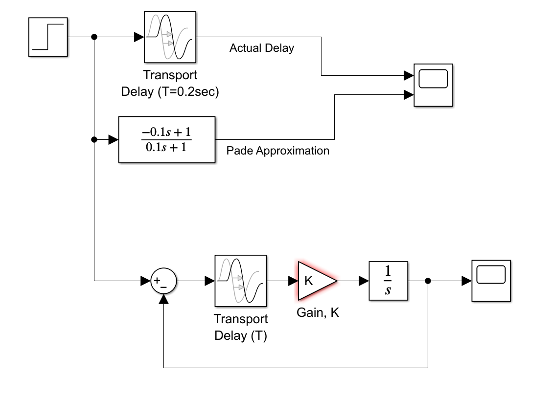
We have been designing our controllers with dynamics elements, including filters, integrators, and derivatives. In our analysis, we represent these using Laplace transforms ("s"), and "pretending" that they exist in the continuous-time world. But as we are discovering in the lab, we almost always implement feedback controllers on a digital computer, and the dynamics happen in "discrete time"-that is, the control calculations take place at a typically fixed interval, and the commands to the actuator are updated only after each calculation. We also use delay to represent the effects of other things that we don't want to model in detail, such as the time it takes actuators and sensors to respond to their inputs. The transfer function of time delay 1 is Gd(s)=eTs. But we like to work with transfer function that are ratios of polynomials in s, so we often use a Pade approximation 2 for time delay, the simplest version of which is Gd(s)2Ts+12Ts+1 Run the provided Simulink model to see how the Pade approximation compares to the actual effects of delay. The step response comparison looks pretty lame, but the Pade approximation turns out to be quite useful for analyzing feedback control. Consider the effects of time delay on a very simple feedback system, shown at the right. If there is no delay (T=0), we find the closed-loop transfer function is simply ydy=s+KK We know that increasing the gain causes the pole to move left, corresponding to a reduction of the closed-loop time constant; the system is stable for all K>0. If we include the exact representation of delay, we get the following closed-loop transfer function: ydy=s+KeTsKeTs And we don't really know what to do with the strange denominator: we can only use root locus analysis on a transfer function with polynomial numerators and denominators. On the other hand, with the Pade approximation, we get the following closed-loop transfer function: ydy=s2+(T2K)s+KT2K(s+T2) There is a negative damping effect of feedback! This model predicts that we reach neutral damping (zero damping ratio) with K=Ku=T2. For example, when T=0.2, the gain for neutral stability is predicted to be Ku=10. a. Use Matlab's rlocus command to make a root locus plot for this system and confirm that Ku=10. b. Use the provided Simulink model to determine what actual gain is required for neutral stability when T=0.2sec. You should discover that the value of Ku is lower than we predicted. This is bad news, because as engineers, we like our analysis to be conservative (or pessimistic): it is better to predict that a stable system is unstable than that an unstable system is stable! Soon we'll see how to get the exact answer for the effects of time delay using frequency response analysis (Bode plots)
Step by Step Solution
There are 3 Steps involved in it

Get step-by-step solutions from verified subject matter experts


