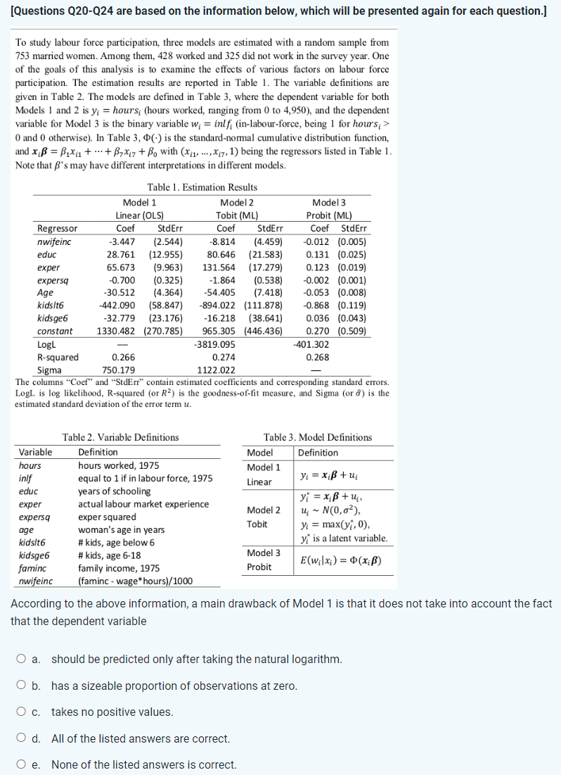
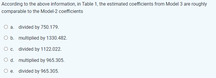
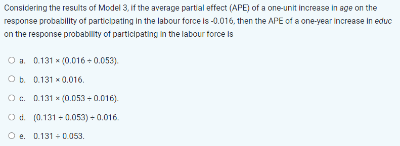
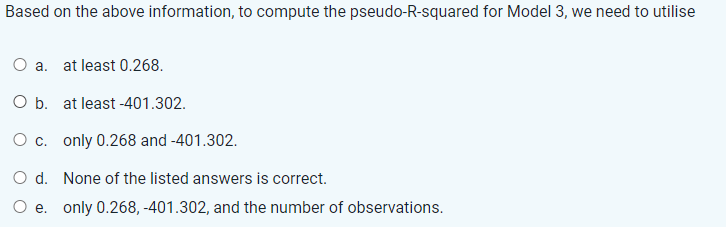
[Questions Q20-Q24 are based on the information below, which will be presented again for each question.] To study labour force participation, three models are estimated with a random sample from 753 married women. Among them, 428 worked and 325 did not work in the survey year. One of the goals of this analysis is to examine the effects of various factors on labour force participation. The estimation results are reported in Table 1. The variable definitions are given in Table 2. The models are defined in Table 3, where the dependent variable for both Models 1 and 2 is y = hours; (hours worked, ranging from 0 to 4,950), and the dependent variable for Model 3 is the binary variable w, = inif, (in-labour-force, being 1 for hours, > 0 and 0 otherwise). In Table 3, 4(.) is the standard-normal cumulative distribution function, and x:B = BiXu+ + Byxi7 + Bo with (Xq. ...*;7, 1) being the regressors listed in Table 1. Note that 's may have different interpretations in different models. Table 1. Estimation Results Model 1 Model 2 Model 3 Linear (OLS) Tobit (ML) Probit (ML) Regressor Coef StdErr Coef StdErr Coef StdErr nwifeinc -3.447 (2.544) 8.814 (4.459) -0.012 (0.005) educ 28.761 (12.955) 80.646 (21.583) 0.131 (0.025) exper 65.673 (9.963) 131.564 (17.279) 0. 123 (0.019) expersq -0.700 (0.325) -1.864 (0.538) 0.002 (0.001) Age -30.512 (4.364) -54.405 (7.418) 0.053 (0.008) kidsit6 442.090 (58.847) -894.022 (111.878) 0.868 (0.119) kidsge6 -32.779 (23.176) -16.218 (38.641) 0.036 (0.043) constant 1330.482 (270.785) 965.305 (446.436) 0.270 (0.509) LogL -3819.095 -401.302 R-squared 0.266 0.274 0.268 Sigma 750.179 1122.022 The columns "Coof" and "StdErr" contain estimated coefficients and corresponding standard errors. LogL is log likelihood, R-squared (or R2) is the goodness-of-fit measure, and Sigma (or o ) is the estimated standard deviation of the error term u. Table 2. Variable Definitions Table 3. Model Definitions Variable Definition Model Definition hours hours worked, 1975 Model 1 inlf equal to 1 if in labour force, 1975 Vi = xiB+ ui Linear educ years of schooling vi = x, B + uj, exper actual labour market experience Model 2 14 ~ N(0, 62), expersq exper squared Tobit Vi = max(yi, 0), age woman's age in years kidsit6 # kids, age below 6 yf is a latent variable. kidsge6 # kids, age 6-18 Model 3 Probit E(wilx) = $(x;B) faminc family income, 1975 nwifeinc (faminc - wage* hours)/1000 According to the above information, a main drawback of Model 1 is that it does not take into account the fact that the dependent variable O a. should be predicted only after taking the natural logarithm. O b. has a sizeable proportion of observations at zero. O c. takes no positive values. O d. All of the listed answers are correct. O e. None of the listed answers is correct.According to the above information, in Table 1, the estimated coefficients from Model 3 are roughly comparable to the Model-2 coefficients P I\\- _'I e divided by 750.179. P 1 1 b = multiplied by 1330.482. P I\\- _'I 3 divided by 1122.022. P 1 1 b o multiplied by 965.305. " L 1 s 1 divided by 965.305. Considering the results of Model 3, if the average partial effect (APE) of a one-unit increase in age on the response probability of participating in the labour force is -0.016, then the APE of a one-year increase in educ on the response probability of participating in the labour force is ) a. 0.131x(0.016 = 0.053). O b. 0.131x0.016. O c. 0.131x(0.053 + 0.016). O d. (0.131+0.053) = 0.016. 0.131 =+ 0.053. P L bt o Based on the above information, for Model 2 the average partial effect (APE) of nwifeinc on the conditional mean of hours (E(hours|X)) is O a. -8.814. O b. -8.814x1122.022. O c. -8.814=1122.022. O d. There is not enough information available to provide an answer. ) e. There is enough information available to provide an answer, but that answer is not listed. Based on the above information, to compute the pseudo-R-squared for Model 3, we need to utilise O a. at least 0.268. O b. at least -401.302. O c. only 0.268 and -401.302. O d. None of the listed answers is correct. O e. only 0.268, -401.302, and the number of observations