R studio, just needs proper formatting
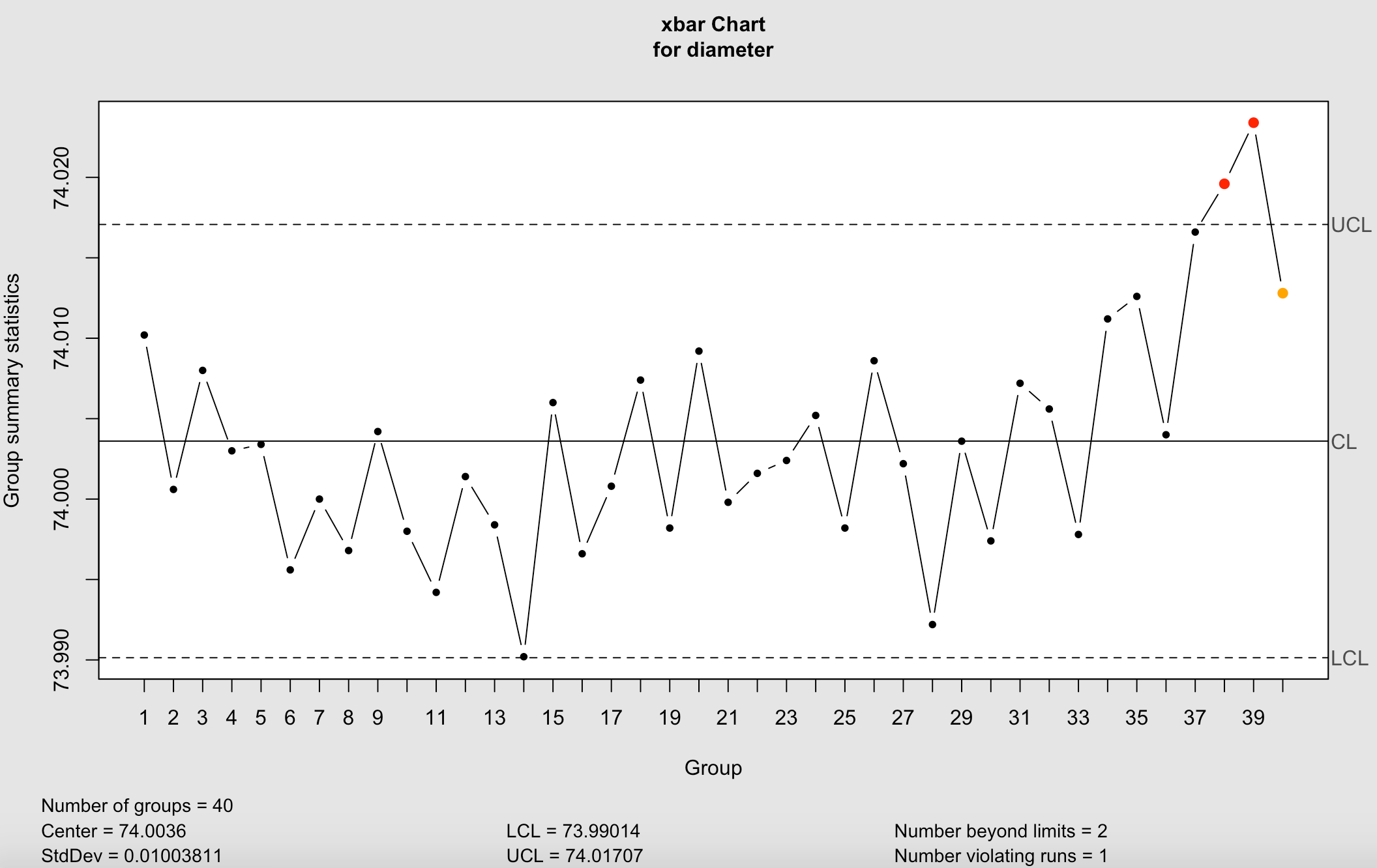
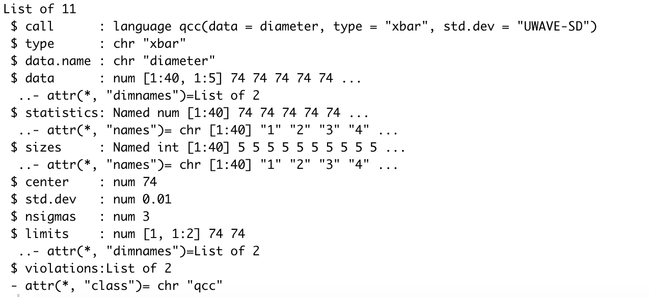
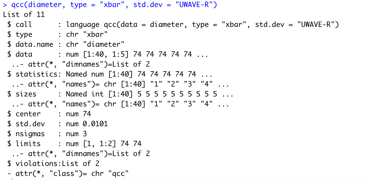
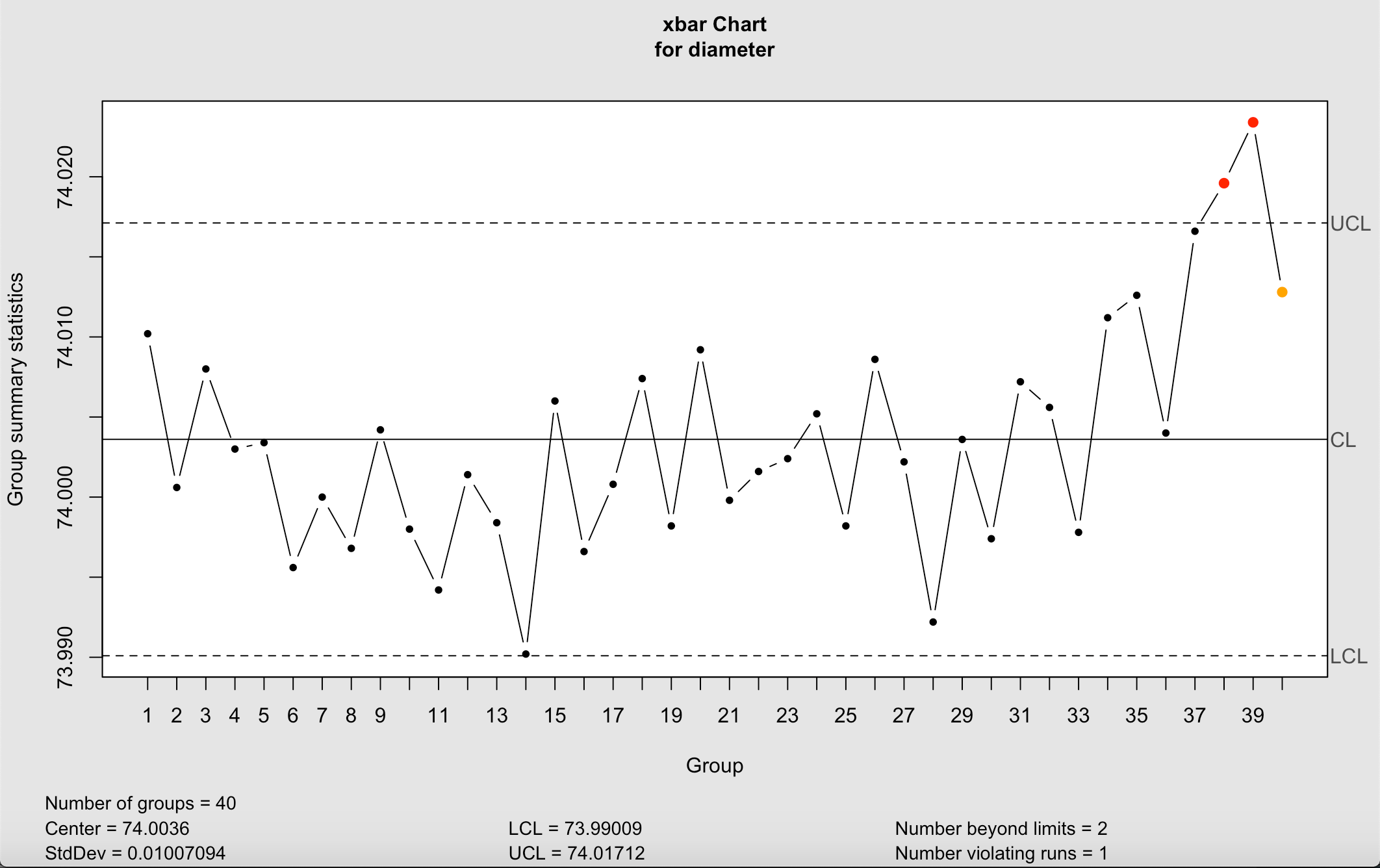
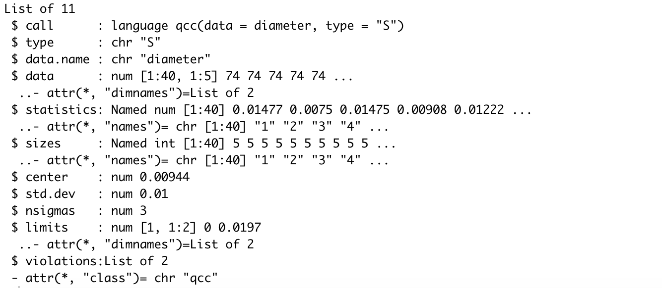
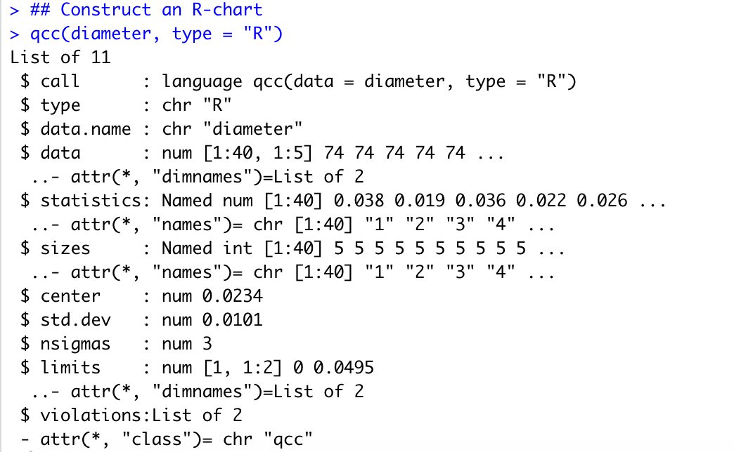
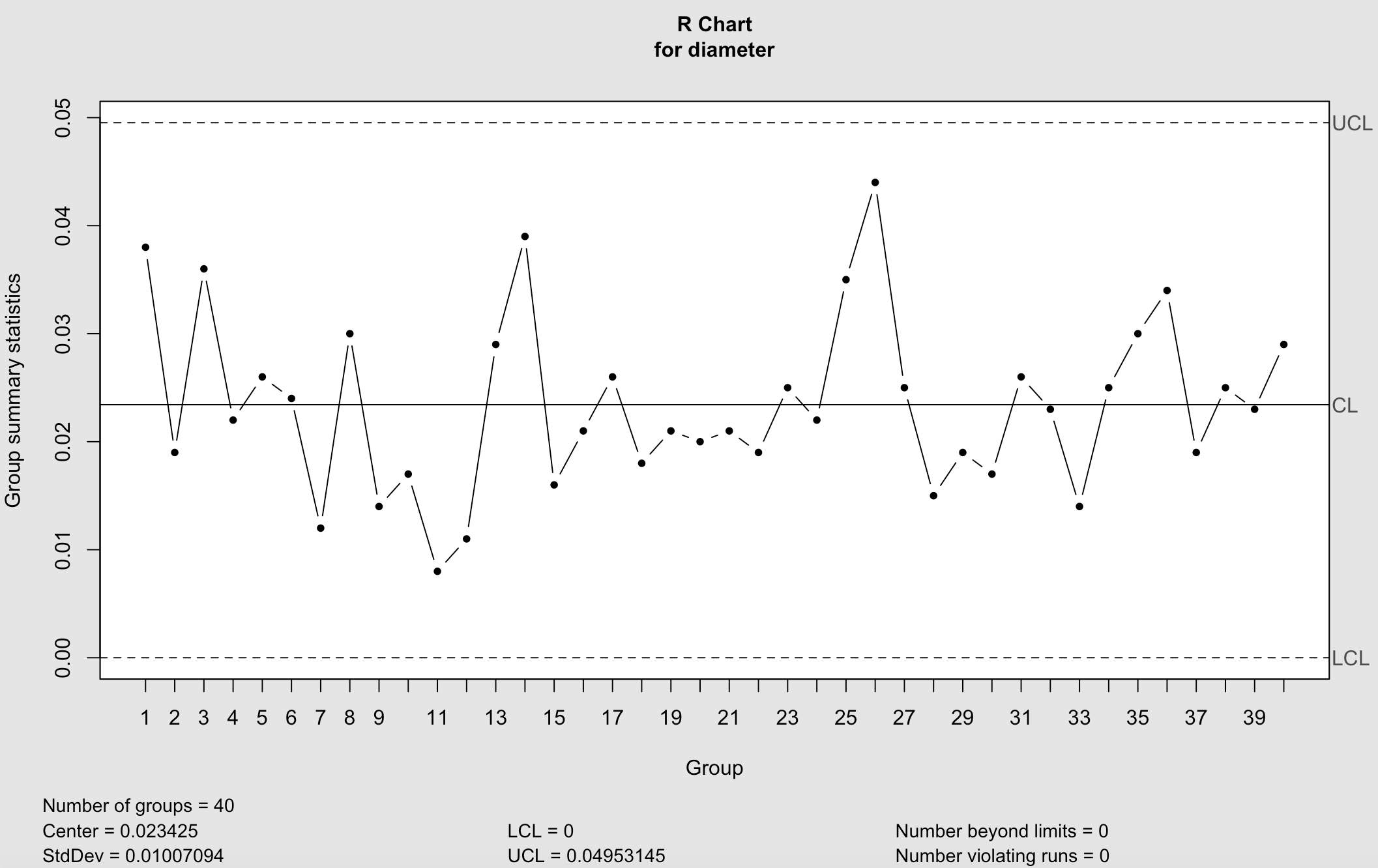
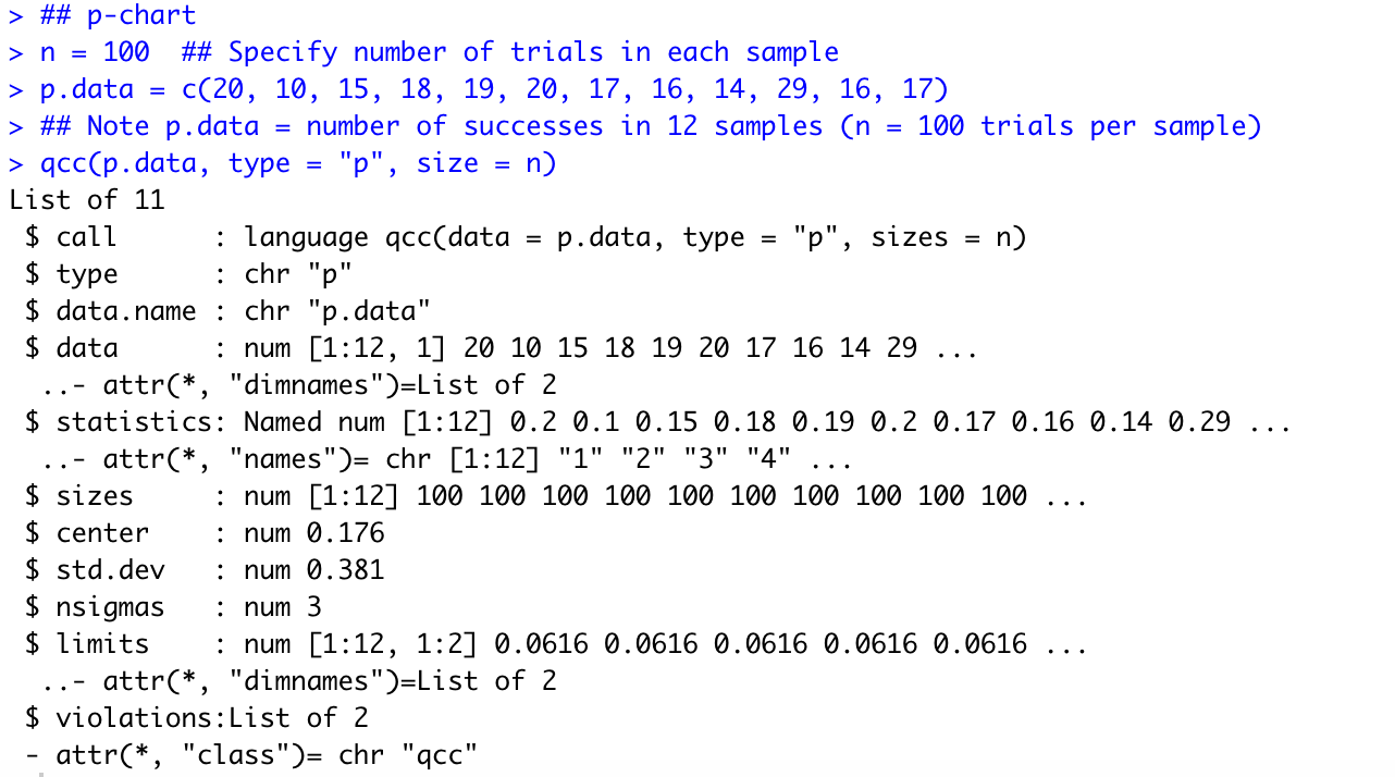
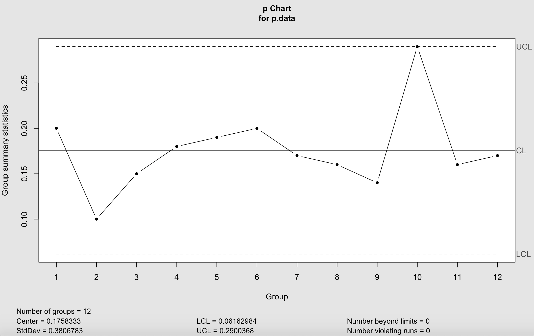
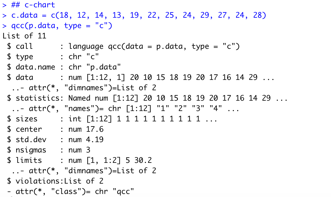
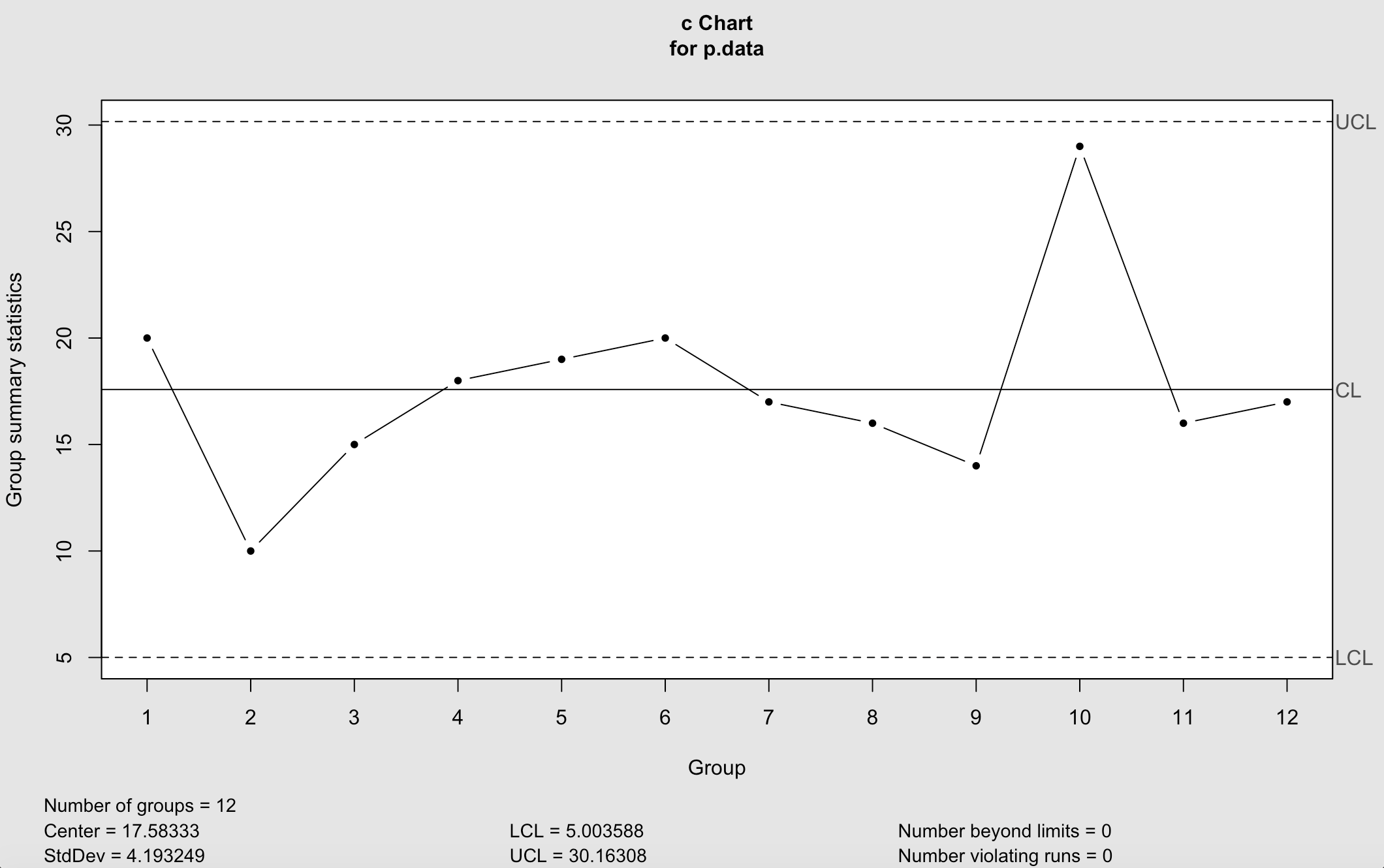
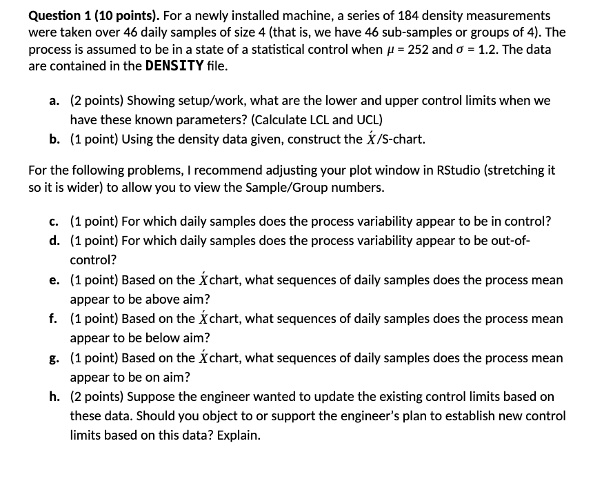
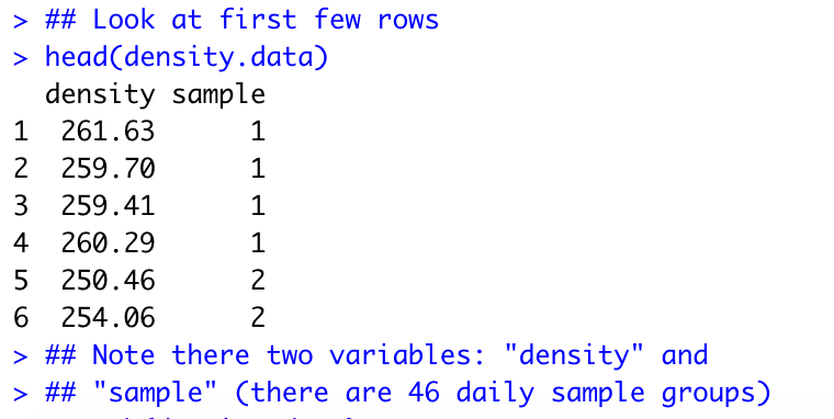
\f\f\f\f\f\f> ## Construct an R-chart > acc(diameter, type = "R") List of 11 $ call : language acc(data = diameter, type = "R") $ type : chr "R" $ data. name : chr "diameter" $ data : num [1:40, 1:5] 74 74 74 74 74 ... . .- attr(*, "dimnames")=List of 2 $ statistics: Named num [1:40] 0. 038 0.019 0. 036 0. 022 0. 026 ... . .- attr(*, "names")= chr [1:40] "1" "2" "3" "4" ... $ sizes : Named int [1:40] 5 5 5 5 5 5 5 5 5 5 ... . .- attr(*, "names")= chr [1:40] "1" "2" "3" "4". $ center : num 0. 0234 $ std. dev : num 0. 0101 $ nsigmas : num 3 $ limits : num [1, 1:2] 0 0. 0495 . .- attr(*, "dimnames")=List of 2 $ violations : List of 2 - attr(*, "class")= chr "qcc"\f> ## p-chart > n = 100 ## Specify number of trials in each sample > p. data = c(20, 10, 15, 18, 19, 20, 17, 16, 14, 29, 16, 17) > ## Note p. data = number of successes in 12 samples (n = 100 trials per sample) > qcc(p. data, type = "p", size = n) List of 11 $ call : language acc(data = p. data, type = "p", sizes = n) $ type : chr "p" $ data. name : chr "p. data" $ data : num [1:12, 1] 20 10 15 18 19 20 17 16 14 29 ... . .- attr(*, "dimnames")=List of 2 $ statistics: Named num [1:12] 0.2 0.1 0.15 0. 18 0. 19 0.2 0. 17 0. 16 0. 14 0.29 ... . .- attr(*, "names")= chr [1:12] "1" "2" "3" "4" .. $ sizes : num [1:12] 100 100 100 100 100 100 100 100 100 100 ... $ center : num 0. 176 $ std. dev : num 0. 381 $ nsigmas : num 3 $ Limits : num [1:12, 1:2] 0. 0616 0. 0616 0. 0616 0. 0616 0.0616 ... . .- attr(*, "dimnames")=List of 2 $ violations : List of 2 - attr(*, "class")= chr "qcc"\f> ## c-chart > c. data = c(18, 12, 14, 13, 19, 22, 25, 24, 29, 27, 24, 28) > qcc(p. data, type = "c") List of 11 $ call : language acc(data = p. data, type = "c") $ type : chr "c" $ data. name : chr "p. data" $ data : num [1:12, 1] 20 10 15 18 19 20 17 16 14 29 ... . .- attr(*, "dimnames")=List of 2 $ statistics: Named num [1:12] 20 10 15 18 19 20 17 16 14 29 ... . .- attr(*, "names")= chr [1:12] "1" "2" "3" "4" ... $ sizes : int [1:12] 1 1 1 1 1 1 1 1 1 1 ... $ center : num 17.6 $ std. dev : num 4. 19 $ nsigmas : num 3 $ limits : num [1, 1:2] 5 30.2 .- attr(*, "dimnames")=List of 2 $ violations : List of 2 attr(*, "class")= chr "qcc"\fQuestion 1 (10 points}. For a newly installed machine, a series of 134 density measurements were taken over 46 daily samples of size 4 (that isI we have 46 sub-samples or groups of 4). The process is assumed to be in a state of a statistical control when ,u = 252 and a = 1.2. The data are contained in the DENSITY le. b. (2 points] Showing setup/work, what are the lower and upper control limits when we have these known parameters? (Calculate LCL and UCL) (1 point) Using the density data given, construct the X/S-chart. For the following problems, I recommend adjusting your plot window in RStudio {stretching it so it is wider) to allow you to view the Sample/Group numbers. c. d. (1 point) For which daily samples does the process variability appear to be in control? (1 point) For which daily samples does the process variability appear to be out-of- control? (1 point) Based on the 12 chart, what sequences of daily samples does the process mean appear to be above aim? (1 point) Based on the 12 chart, what sequences of daily samples does the process mean appear to be below aim? (1 point) Based on the if chart, what sequences of daily samples does the process mean appear to be on aim? (2 points) Suppose the engineer wanted to update the existing control limits based on these data. Should you object to or support the engineer's plan to establish new control limits based on this data? Explain. > ## Look at first few rows > head(density . data) density sample 1 261.63 259 . 70 259 .41 4 260.29 5 250.46 6 254. 06 NNPPPP > ## Note there two variables: "density" and > ## "sample" (there are 46 daily sample groups)