Refer to Section 2.4.9 given in the course text on pages 31-33. This example refers to the results given in Figure 2.14 that were produced by solving the model eqs. 2-98 to 2-101 using a numerical integration method with the model parameters and two sets of initial conditions listed in Table 2.3 on page 33. The assignment is to write a Matlab code (and not a Polymath code) that reproduces the results shown in the above-referenced figures. There are two cases shown, namely, those at F = 0.05 L/hr and another set at F = 0.02 L/hr. The methodology is similar to what was done in one of the early lab exercises where we created a MATLAB code to numerically solve ODEs. If needed, refer to this exercise and follow a similar procedure. Your solution package should consist of the following.

(a) A summary of the model assumptions and starting ODE model equations and the various initial conditions that were used to generate each of the results. Do not derive the equations, but use them directly as given. Show that the units for the various parameters that are given are consistent.

(b) A table that shows the actual variable that appears in the model equations and the corresponding computer-based variable. For example, the model variable rP may be written as rP while the model variable Sf may be written in your code Ssubf.

(c) Listing of the Matlab codes that were used to generate the sub-plots shown in Figure 2.14

(d) A copy of the figures that are formatted like those shown in Figure 2.14

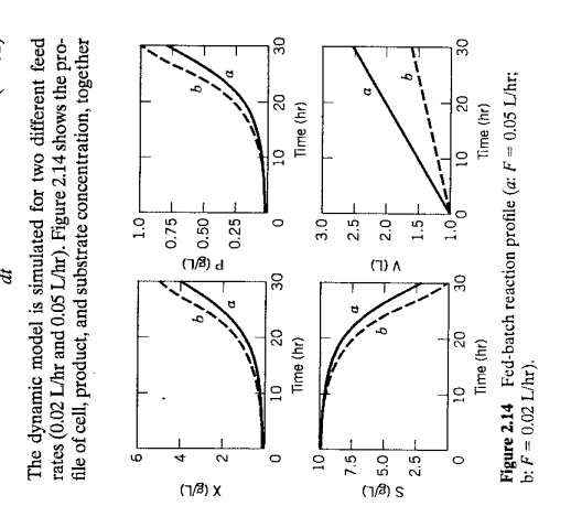
fig 2.14

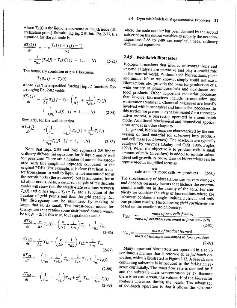
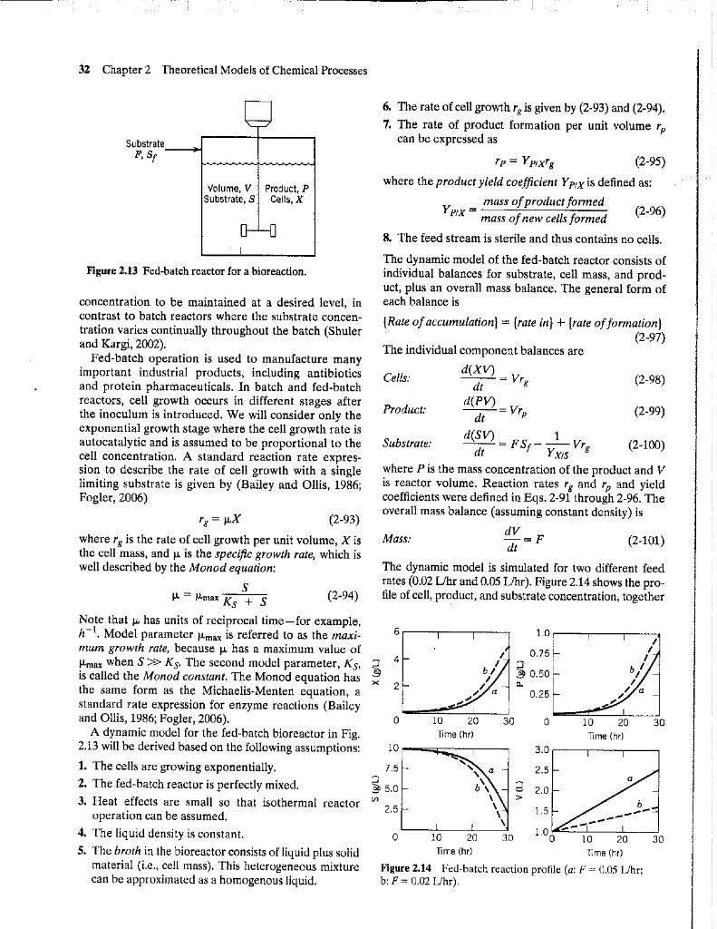
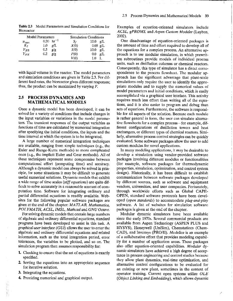
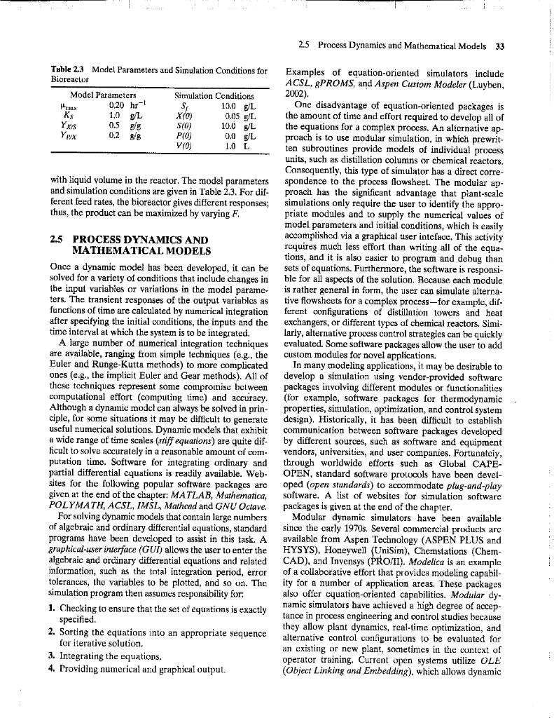
The dynamic model is simulated for two different feed rates ( 0.02L/hr and 0.05L/hr). Figure 2.14 shows the profile of cell, product, and substrate concentration, together Figure 2.14 Fed-batch reaction profile (a:F=0.05L/hr; b: F=0.02L/hr, 2.4 Dynamic Models of Representative Processes 31 where TL(j) is the liquid temperatire at the j th node (dis- where the node number has been denoted by the second cretization point). Substituting Eq. 2-81 into Eq. 2-77, the subscript on the output variables to simplify the notation. equation for the j th node is dtdTL(j)=vzTL(j)TL(j1)+HL1[Tw(j)TL(j)](j=1,,M) Equations 2-86 to 2-89 are coupled, linear, ordinary differential equations. 2.4.9 Fed-Batch Bioreactor (2-82) Biological reactions that involve microorganisms and Theboundaryconditionatz=0becomesinthenaturalworld.Withoutsuchbioreactions,plantenzymecatalystsarepervasiveandplayacrucialrole TL(0,t)=TF(t) (2-83) and animal life as we know it simply could not exist. where TF(t) is a specified forcing (input) function. Re - Bioreactions also provide the basis for production of a arranging Eq. 2-82 yields dTL(j) food products. Other important industrial processes that involve bioreactions include fermentation and wastewater treatment. Chemical engineers are heavily involved with biochemical and biomedical processes. In (2-84) this section we present a dynamic model for a representative process, a bioreactor operated in a semi-batch mode. Additional biochemical and biomedical applications appear in other chapters. In general, bioreactions are characterized by the conversion of feed material (or substrate) into products Note that Eqs, 284 and 285 represent 2N catalyzed by enzymes (Bailey and Ollis, 1986; Fogler, ordinary differential equations for N liquid and N wall amount of cells (inoculum) is added to initiate subsetemperatures. There are a number of anomalies associ- quent cell growth. A broad class of bioreactions can be ated with this simplified approach compared to the represented in simplified form as the zeroth node (the entrance), but is accounted for at The stoichiometry of bioreactions can be very complex all other nodes. Also, a detailed analysis of the discrete and depends on many factors that include the environmodel will show that the steady-state relations between mental conditions in the vicinity of the cells. For simTL(j) and either input, Tg or TF, are a function of the plicity we consider the class of bioreactions where the number of grid points and thus the grid spacing. z. substrate contains a single limiting nutrient and only The discrepancy can be minimized by making N one product results. The following yield coefficients are large, that is, z small, The lowest-order model for based on the reaction stoichiometry: this system that retains some distribtated nature would be for N=2. In this case, four equations result: dtdTL1=zvTF(t)(zv+HL1)TL1+HL1Tw1YXiS=massofsubstrateconsumedtoformnewcellsmassofnewcellsformed (2-96) 91) dTL2=YPSSv=massofsubstrateconsumedtoformproductmassofproductformed dtdTL2=zvTL1(zv+HL1)TL2+HL1TH2 (2-92) (2-87) Many important bioreactors are operated in a semidTw1(1)1) continuouts manner that is referred to as fed-batch operation, which is illustrated in Figure 2.13. A feed stream containing substrate is introduced to the fed-batch re(2-88) actor continually. The mass flow rate is denoted by F and the substrate mass concentration by Sf Because there is no exit stream, the volume V of the bioreactor contents increases during the batch. The advantage (2-89) of fed-batch operation is that it allows the substrate 32 Chapter 2 Theoretical Models of Chemical Processes 6. The rate of cell growth rg is given by (2-93) and (2-94). 7. The rate of product formation per unit volume rp can be expressed as rP=YPHXrg where the product yield coefficient YPtX is defined as: YPXX=massofnewcellsformedmassofproductformed 8. The feed stream is sterile and thus contains no cells. The dynamic model of the fed-batch reactor consists of Figure 2,13 Fed-batch rcactor for a bioreaction. individual balances for substrate, cell mass, and product, plus an overall mass balance. The general form of concentration to be maintained at a desired level, in each balance is tration varics continually throughout the batch (Shuler { Rate of accumulation }={ rate in }+{ rate of formation } and Kargi, 2002). (2-97) Fed-batch operation is used to manufacture many important industrial products, including antibiotics and protein pharmaceuticals. In batch and fed-batch Cells: dtd(XV)=Vrg reactors, cell growth occurs in different stages after the inoculum is introduced. We will consider only the Product: dtd(PV)=Vrp exponential growth stage where the cell growth rate is autocatalytic and is assumed to be proportional to the cell concentration. A standard reaction rate expression to describe the rate of cell growth with a single where P is the mass concentration of the product and V limiting substrate is given by (Bailey and Ollis, 1986; is reactor volume. Reaction rates rg and rp and yield Fogler, 2006) coefficients were defined in Eqs. 2-91 through 2-96. The rg=X (2-93) overall mass balance (assuming constant density) is where rg is the rate of cell growth per unit volume, X is Mass: dtdV=F (2101) the cell mass, and is the specific growth rate, which is well described by the Monod equation: The dynamic model is simulated for two different feed =maxKS+SS (2-94) fates (0.02L/hr and 0.05L/hr). Figure 2.14 shows the pro- Note that has units of reciprocal time-for example, h1. Model parameter max is referred to as the maximum growth rate, because has a maximum value of max when SKS. The second model parameter, KS+, is called the Monod constant. The Monod equation has the same form as the Michaelis-Menter equation, a standard rate expression for enzyme reactions (Bailcy and Otlis, 1986; Fogler, 2006). A dynamic model for the fed-batch bioreactor in Fig. 2.13 will be derived based on the following assumptions: 1. The cells are growing exponentially. 2. The fed-batch reactor is perfectly mixed. 3. Heat effects are small so that isothermal reactor operation can be assumed. 4. The liquid density is constant. 5. The broth ia the bioreactor consists of liquid plus solid material (i.e., cell mass). This heterogeneous mixture Figure 2.14 Fed-batch reaction profile (a: F=0.05Lhr; can be approximated as a homogenous liquid. b:F=0.02L/hr ). Table 2.3 Model Parameters and Simulation Conditions for Examples of equation-oriented simulators include Bioreactor ACSL, gPROMS, and Aspen Custom Modeler (Luyben, 2002). One disadvantage of equation-oriented packages is the amount of time and effort required to develop all of the equations for a complex process. An alternative approach is to use modular simulation, in which prewritten subroutines provide models of individual process units, such as distillation columns or chemical reactors. Consequently, this type of simulator has a direct correwith liquid volume in the reactor. The model parameters spondence to the process llowshcet. The modular apand simulation conditions are given in Table 2.3. For dif- proach has the significant advantage that plant-scale ferent feed rates, the bioreactor gives different responses; simulations only require the user to identify the approthus, the product can be maximized by varying F. priate modules and to supply the numerical values of model parameters and initial conditions, which is easily 2.5 PROCESS DYNAMICS AND accomplished via a graphical user inteface. This activity MATHEMATICALMODELS requires much less effort than writing all of the equaOnce a dynamic model has been developed, it can be thons, and it is also easier to program and debug than solved for a variety of conditions that include changes in ble for all aspects of the soiution. Beceuse cach module the input variables or variations in the model parame- is rather general in form, the user can simulate alternaters. The transicnt responses of the output variables as tive flowshcets for a complex procoss-for example, diffunctions of time are calculated by numerical integration. ferent configurations of distillation towers and heat after specifying the initial conditions, the inputs and the exchangers, or different types of chemical reactors. Simitime interval at which the system is to be integrated. larly, alternative process control strategies can be quickly A large number of numerical integration techniques evaluated, Some software packages allow the user to add are available, ranging from simple techniques (e,ga, the custom modules for novel applications. Euler and Runge-Kutta methods) to more complicated In many modeling applications, it may be desirable to otles (e.g., the implicit Euler and Gear methods). All of develop a simulation using vendor-prowided software these techniques represent some compromise between packages involving difterent modules or functionalities computational effort (computing time) and accuracy. (for example, software packages for thermodynamic Although a dynamic model can always be solved in prin- properties, simulation, optimization, and control system ciple, for some situations it may be difficult to generate design). Historically, it has been difficult to establish useful numerical solutions. Dynamic models that exhibit communication between software packages developed a wide range of time scales (stiff equations) are quite dif- by different sources, such as software and equipment ficult to solve accurately in a reasonable amount of com- vendors, universities, and user companies. Fortunately, putation time. Software for integrating ordinary and through worldwide efforts such as Global CAPEpartial differential equations is readily available. Web- OPEN, standard software protocols have been develsites for the following popular software packages are oped (open standards) to accommodate plug-and-play' given at the end of the chapter: MATLAB, Marhematica, software. A list of websites for simulation software POLYMATH, ACSL, IMSL, Mathcad and GNUOctave packages is given at the enc of the chapter. For solving dynamis models that contain large numbers Modular dynamic simulators have been available of algebraic and ordinary differential equations, standard since the early 1970 s. Several commercial products are programs have been developed to assist in this task. A available from Aspen Technology (ASPEN PLUS and graphical-user interface (GUI) allows the user to enter the HYSYS), Honeywell (UniSim), Chemstations (Chemalgebraic and ordinary differential equations and related CAD), and Invensys (PRO/II). Modelica is an example information, such as the total integration period, error of a collaborative effort that provides modeling capabiltolerances, the variables to be plotted, and so on. The ity for a number of application areas. These packages simulation program ther assumes responsibility for: also offer equation-oriented capabilities. Modular dy- 1. Checking to ensure that the set of equations is exactly namic simulators have achieved a high degree of accepspecified. 2. Sorting the equations into ar appropriate sequence they allow plant dynamics, real-time optimization, and for iterative solution. alternative control configurations to be evaluated for 3. Integrating an existing or new plant, sometimes in the context of 3. Integrating the equations. operator training. Current open systems utilize OLE 4. Providing numerical and graphical output. (Object Linking and Enbedding), which allows dynamic 2.5 Process Dynamics and Mathematical Models 33 Tuble 2.3 Model Parameters and Simulation Conditions for Examples of equation-oriented simulators include Bioreactot ACSL, gPROMS, and Aspen Custom Modeler (Luyben, 2002) One disadvantage of equation-oriented packages is the amount of time and effort required to develop tll of the equations for a complex process. An aliernative approach is to use modular simulation, in which prewritten subroutines provide models of individual process units, such as distillation columns or chemical reactors. Consequently, this type of simulator has a direct correwith liquid volume in the reactor. The model parameters spondence to the process flowsheet. The moduiar apand simulation conditions are given in Table 2.3. For dif- proach has the significant advantage that plant-scale ferent feed rates, the bioreactor gives different responses; simulations only require the user to identify the approthus, the product can be maximized by varying F. priate modules and to supply the numerical values of model parameters and initial conditions, which is easily 2.5 PROCESS DYNAMICS ANI aceomplished via a graphical user inteface. This activity MATHEMATICAL MODELS rcquires much less effort than writing all of the equaOnce a dynamic model has been developed, it can be tions, and it is also easier to program and debug than solved for a variety of conditions that include changes in sets of equations. Furthermore, the software is responsithe input variables or variations in the model parame- ble for all aspects of the solution. Because each module ters. The transient responses of the output varib is rather general in form, the user can simulate alternafunctions of time are calculated by nump tive flowsheets for a complex process-for example, difafter specifying the furent configurations of distillation towers and heat time intersal the initial conditions, the inputs and the exchangers, or different types of chemical reactors, SimiA large number of system is to be integrated. lariy, alternative process control strategies can be quickly are available, ram of numerical integration techniques evaluated. Some software packages allow the user to add are avallable, ranging from simple techniques (e.g., the custom modules for novel applications. Euler and Runge-Kutta methods) to more complicated In many modeling applications, it may be desirable to ones (e.g., the implicit Euler and Gear methods). All of develop a simulation using vendor-provided software these techniques represent some compromise between packages involving different modules or functionalities computational effort (computing time) and accuracy. (for example, software packages for thermodynamic Although a dynamic model can always be solved in prin- properties, simulation, optimization, and control system ciple, for some situations it may be difficult to generate design). Historicaliy, it has been difficult to establish useful numerical solutions. Dynamic models that exhibit communication between software packages developed a wide range of time scales (stiff equations) are quite dif- by different sources, such as software and equipment ficult to solve accurately in a reasonable amount of com- vendors, universities, and user companies. Fortanateiy, putation time. Software for integrating ordinary and through worldwide efforts such as Global CAPEpartial differential equations is readily available. Web- OPEN, standard software protocols have been develsites for the following popular software packages are oped (open standards) to accommodate plug-and-play given at the end of the chapter: MATLAB, Mathematica, software. A list of websites for simulation software POLYMATH, ACSL, IMSL, Mathcad and GNUOctave. packages is given at the end of the chapter. For solving dynamic models that contain large numbers Modular dynamic simulators have been available of algebraic and ordinary differential equations, standard sitce the early 1970 s. Several commercial products are programs have been developed to assist in this task. A available from Aspen Technology (ASPEN PLUS and graphical-user interface (GUI) allows the user to enter the HYSYS). Honeywell (UniSim), Chemstations (Chemalgebraic and orcinary differential equations and related CAD), and Invensys (PRO/II). Modelica is an example information, such as the total integration period, error of a collaborative effort that provides modeling capabiltolerances, the variables to be plotted, and so on. The ity for a number of application areas. These packages simulation program then assumes responsibility for: also offer equation-oriented capabilities. Moduiar dy- 1. Checking to ensure that the set of equations is exactly namic simulators have achieved a high degree of accepspecified. 2. Sorting the equations into an appropriate sequence they allow plant dynamics, real-time optimization, and for iterative solution. alternative control congurations to be evaluated for 3. Integrating the an existing or new plant, sometimes in the context of 4. Integrating the equations. operator training. Current open systems utilize OLE 4. Providing numerical and graphical output. (Object Linking and Embedding), which allows dynamic The dynamic model is simulated for two different feed rates ( 0.02L/hr and 0.05L/hr). Figure 2.14 shows the profile of cell, product, and substrate concentration, together Figure 2.14 Fed-batch reaction profile (a:F=0.05L/hr; b: F=0.02L/hr, 2.4 Dynamic Models of Representative Processes 31 where TL(j) is the liquid temperatire at the j th node (dis- where the node number has been denoted by the second cretization point). Substituting Eq. 2-81 into Eq. 2-77, the subscript on the output variables to simplify the notation. equation for the j th node is dtdTL(j)=vzTL(j)TL(j1)+HL1[Tw(j)TL(j)](j=1,,M) Equations 2-86 to 2-89 are coupled, linear, ordinary differential equations. 2.4.9 Fed-Batch Bioreactor (2-82) Biological reactions that involve microorganisms and Theboundaryconditionatz=0becomesinthenaturalworld.Withoutsuchbioreactions,plantenzymecatalystsarepervasiveandplayacrucialrole TL(0,t)=TF(t) (2-83) and animal life as we know it simply could not exist. where TF(t) is a specified forcing (input) function. Re - Bioreactions also provide the basis for production of a arranging Eq. 2-82 yields dTL(j) food products. Other important industrial processes that involve bioreactions include fermentation and wastewater treatment. Chemical engineers are heavily involved with biochemical and biomedical processes. In (2-84) this section we present a dynamic model for a representative process, a bioreactor operated in a semi-batch mode. Additional biochemical and biomedical applications appear in other chapters. In general, bioreactions are characterized by the conversion of feed material (or substrate) into products Note that Eqs, 284 and 285 represent 2N catalyzed by enzymes (Bailey and Ollis, 1986; Fogler, ordinary differential equations for N liquid and N wall amount of cells (inoculum) is added to initiate subsetemperatures. There are a number of anomalies associ- quent cell growth. A broad class of bioreactions can be ated with this simplified approach compared to the represented in simplified form as the zeroth node (the entrance), but is accounted for at The stoichiometry of bioreactions can be very complex all other nodes. Also, a detailed analysis of the discrete and depends on many factors that include the environmodel will show that the steady-state relations between mental conditions in the vicinity of the cells. For simTL(j) and either input, Tg or TF, are a function of the plicity we consider the class of bioreactions where the number of grid points and thus the grid spacing. z. substrate contains a single limiting nutrient and only The discrepancy can be minimized by making N one product results. The following yield coefficients are large, that is, z small, The lowest-order model for based on the reaction stoichiometry: this system that retains some distribtated nature would be for N=2. In this case, four equations result: dtdTL1=zvTF(t)(zv+HL1)TL1+HL1Tw1YXiS=massofsubstrateconsumedtoformnewcellsmassofnewcellsformed (2-96) 91) dTL2=YPSSv=massofsubstrateconsumedtoformproductmassofproductformed dtdTL2=zvTL1(zv+HL1)TL2+HL1TH2 (2-92) (2-87) Many important bioreactors are operated in a semidTw1(1)1) continuouts manner that is referred to as fed-batch operation, which is illustrated in Figure 2.13. A feed stream containing substrate is introduced to the fed-batch re(2-88) actor continually. The mass flow rate is denoted by F and the substrate mass concentration by Sf Because there is no exit stream, the volume V of the bioreactor contents increases during the batch. The advantage (2-89) of fed-batch operation is that it allows the substrate 32 Chapter 2 Theoretical Models of Chemical Processes 6. The rate of cell growth rg is given by (2-93) and (2-94). 7. The rate of product formation per unit volume rp can be expressed as rP=YPHXrg where the product yield coefficient YPtX is defined as: YPXX=massofnewcellsformedmassofproductformed 8. The feed stream is sterile and thus contains no cells. The dynamic model of the fed-batch reactor consists of Figure 2,13 Fed-batch rcactor for a bioreaction. individual balances for substrate, cell mass, and product, plus an overall mass balance. The general form of concentration to be maintained at a desired level, in each balance is tration varics continually throughout the batch (Shuler { Rate of accumulation }={ rate in }+{ rate of formation } and Kargi, 2002). (2-97) Fed-batch operation is used to manufacture many important industrial products, including antibiotics and protein pharmaceuticals. In batch and fed-batch Cells: dtd(XV)=Vrg reactors, cell growth occurs in different stages after the inoculum is introduced. We will consider only the Product: dtd(PV)=Vrp exponential growth stage where the cell growth rate is autocatalytic and is assumed to be proportional to the cell concentration. A standard reaction rate expression to describe the rate of cell growth with a single where P is the mass concentration of the product and V limiting substrate is given by (Bailey and Ollis, 1986; is reactor volume. Reaction rates rg and rp and yield Fogler, 2006) coefficients were defined in Eqs. 2-91 through 2-96. The rg=X (2-93) overall mass balance (assuming constant density) is where rg is the rate of cell growth per unit volume, X is Mass: dtdV=F (2101) the cell mass, and is the specific growth rate, which is well described by the Monod equation: The dynamic model is simulated for two different feed =maxKS+SS (2-94) fates (0.02L/hr and 0.05L/hr). Figure 2.14 shows the pro- Note that has units of reciprocal time-for example, h1. Model parameter max is referred to as the maximum growth rate, because has a maximum value of max when SKS. The second model parameter, KS+, is called the Monod constant. The Monod equation has the same form as the Michaelis-Menter equation, a standard rate expression for enzyme reactions (Bailcy and Otlis, 1986; Fogler, 2006). A dynamic model for the fed-batch bioreactor in Fig. 2.13 will be derived based on the following assumptions: 1. The cells are growing exponentially. 2. The fed-batch reactor is perfectly mixed. 3. Heat effects are small so that isothermal reactor operation can be assumed. 4. The liquid density is constant. 5. The broth ia the bioreactor consists of liquid plus solid material (i.e., cell mass). This heterogeneous mixture Figure 2.14 Fed-batch reaction profile (a: F=0.05Lhr; can be approximated as a homogenous liquid. b:F=0.02L/hr ). Table 2.3 Model Parameters and Simulation Conditions for Examples of equation-oriented simulators include Bioreactor ACSL, gPROMS, and Aspen Custom Modeler (Luyben, 2002). One disadvantage of equation-oriented packages is the amount of time and effort required to develop all of the equations for a complex process. An alternative approach is to use modular simulation, in which prewritten subroutines provide models of individual process units, such as distillation columns or chemical reactors. Consequently, this type of simulator has a direct correwith liquid volume in the reactor. The model parameters spondence to the process llowshcet. The modular apand simulation conditions are given in Table 2.3. For dif- proach has the significant advantage that plant-scale ferent feed rates, the bioreactor gives different responses; simulations only require the user to identify the approthus, the product can be maximized by varying F. priate modules and to supply the numerical values of model parameters and initial conditions, which is easily 2.5 PROCESS DYNAMICS AND accomplished via a graphical user inteface. This activity MATHEMATICALMODELS requires much less effort than writing all of the equaOnce a dynamic model has been developed, it can be thons, and it is also easier to program and debug than solved for a variety of conditions that include changes in ble for all aspects of the soiution. Beceuse cach module the input variables or variations in the model parame- is rather general in form, the user can simulate alternaters. The transicnt responses of the output variables as tive flowshcets for a complex procoss-for example, diffunctions of time are calculated by numerical integration. ferent configurations of distillation towers and heat after specifying the initial conditions, the inputs and the exchangers, or different types of chemical reactors. Simitime interval at which the system is to be integrated. larly, alternative process control strategies can be quickly A large number of numerical integration techniques evaluated, Some software packages allow the user to add are available, ranging from simple techniques (e,ga, the custom modules for novel applications. Euler and Runge-Kutta methods) to more complicated In many modeling applications, it may be desirable to otles (e.g., the implicit Euler and Gear methods). All of develop a simulation using vendor-prowided software these techniques represent some compromise between packages involving difterent modules or functionalities computational effort (computing time) and accuracy. (for example, software packages for thermodynamic Although a dynamic model can always be solved in prin- properties, simulation, optimization, and control system ciple, for some situations it may be difficult to generate design). Historically, it has been difficult to establish useful numerical solutions. Dynamic models that exhibit communication between software packages developed a wide range of time scales (stiff equations) are quite dif- by different sources, such as software and equipment ficult to solve accurately in a reasonable amount of com- vendors, universities, and user companies. Fortunately, putation time. Software for integrating ordinary and through worldwide efforts such as Global CAPEpartial differential equations is readily available. Web- OPEN, standard software protocols have been develsites for the following popular software packages are oped (open standards) to accommodate plug-and-play' given at the end of the chapter: MATLAB, Marhematica, software. A list of websites for simulation software POLYMATH, ACSL, IMSL, Mathcad and GNUOctave packages is given at the enc of the chapter. For solving dynamis models that contain large numbers Modular dynamic simulators have been available of algebraic and ordinary differential equations, standard since the early 1970 s. Several commercial products are programs have been developed to assist in this task. A available from Aspen Technology (ASPEN PLUS and graphical-user interface (GUI) allows the user to enter the HYSYS), Honeywell (UniSim), Chemstations (Chemalgebraic and ordinary differential equations and related CAD), and Invensys (PRO/II). Modelica is an example information, such as the total integration period, error of a collaborative effort that provides modeling capabiltolerances, the variables to be plotted, and so on. The ity for a number of application areas. These packages simulation program ther assumes responsibility for: also offer equation-oriented capabilities. Modular dy- 1. Checking to ensure that the set of equations is exactly namic simulators have achieved a high degree of accepspecified. 2. Sorting the equations into ar appropriate sequence they allow plant dynamics, real-time optimization, and for iterative solution. alternative control configurations to be evaluated for 3. Integrating an existing or new plant, sometimes in the context of 3. Integrating the equations. operator training. Current open systems utilize OLE 4. Providing numerical and graphical output. (Object Linking and Enbedding), which allows dynamic 2.5 Process Dynamics and Mathematical Models 33 Tuble 2.3 Model Parameters and Simulation Conditions for Examples of equation-oriented simulators include Bioreactot ACSL, gPROMS, and Aspen Custom Modeler (Luyben, 2002) One disadvantage of equation-oriented packages is the amount of time and effort required to develop tll of the equations for a complex process. An aliernative approach is to use modular simulation, in which prewritten subroutines provide models of individual process units, such as distillation columns or chemical reactors. Consequently, this type of simulator has a direct correwith liquid volume in the reactor. The model parameters spondence to the process flowsheet. The moduiar apand simulation conditions are given in Table 2.3. For dif- proach has the significant advantage that plant-scale ferent feed rates, the bioreactor gives different responses; simulations only require the user to identify the approthus, the product can be maximized by varying F. priate modules and to supply the numerical values of model parameters and initial conditions, which is easily 2.5 PROCESS DYNAMICS ANI aceomplished via a graphical user inteface. This activity MATHEMATICAL MODELS rcquires much less effort than writing all of the equaOnce a dynamic model has been developed, it can be tions, and it is also easier to program and debug than solved for a variety of conditions that include changes in sets of equations. Furthermore, the software is responsithe input variables or variations in the model parame- ble for all aspects of the solution. Because each module ters. The transient responses of the output varib is rather general in form, the user can simulate alternafunctions of time are calculated by nump tive flowsheets for a complex process-for example, difafter specifying the furent configurations of distillation towers and heat time intersal the initial conditions, the inputs and the exchangers, or different types of chemical reactors, SimiA large number of system is to be integrated. lariy, alternative process control strategies can be quickly are available, ram of numerical integration techniques evaluated. Some software packages allow the user to add are avallable, ranging from simple techniques (e.g., the custom modules for novel applications. Euler and Runge-Kutta methods) to more complicated In many modeling applications, it may be desirable to ones (e.g., the implicit Euler and Gear methods). All of develop a simulation using vendor-provided software these techniques represent some compromise between packages involving different modules or functionalities computational effort (computing time) and accuracy. (for example, software packages for thermodynamic Although a dynamic model can always be solved in prin- properties, simulation, optimization, and control system ciple, for some situations it may be difficult to generate design). Historicaliy, it has been difficult to establish useful numerical solutions. Dynamic models that exhibit communication between software packages developed a wide range of time scales (stiff equations) are quite dif- by different sources, such as software and equipment ficult to solve accurately in a reasonable amount of com- vendors, universities, and user companies. Fortanateiy, putation time. Software for integrating ordinary and through worldwide efforts such as Global CAPEpartial differential equations is readily available. Web- OPEN, standard software protocols have been develsites for the following popular software packages are oped (open standards) to accommodate plug-and-play given at the end of the chapter: MATLAB, Mathematica, software. A list of websites for simulation software POLYMATH, ACSL, IMSL, Mathcad and GNUOctave. packages is given at the end of the chapter. For solving dynamic models that contain large numbers Modular dynamic simulators have been available of algebraic and ordinary differential equations, standard sitce the early 1970 s. Several commercial products are programs have been developed to assist in this task. A available from Aspen Technology (ASPEN PLUS and graphical-user interface (GUI) allows the user to enter the HYSYS). Honeywell (UniSim), Chemstations (Chemalgebraic and orcinary differential equations and related CAD), and Invensys (PRO/II). Modelica is an example information, such as the total integration period, error of a collaborative effort that provides modeling capabiltolerances, the variables to be plotted, and so on. The ity for a number of application areas. These packages simulation program then assumes responsibility for: also offer equation-oriented capabilities. Moduiar dy- 1. Checking to ensure that the set of equations is exactly namic simulators have achieved a high degree of accepspecified. 2. Sorting the equations into an appropriate sequence they allow plant dynamics, real-time optimization, and for iterative solution. alternative control congurations to be evaluated for 3. Integrating the an existing or new plant, sometimes in the context of 4. Integrating the equations. operator training. Current open systems utilize OLE 4. Providing numerical and graphical output. (Object Linking and Embedding), which allows dynamic