

Answered step by step
Verified Expert Solution
Question
1 Approved Answer
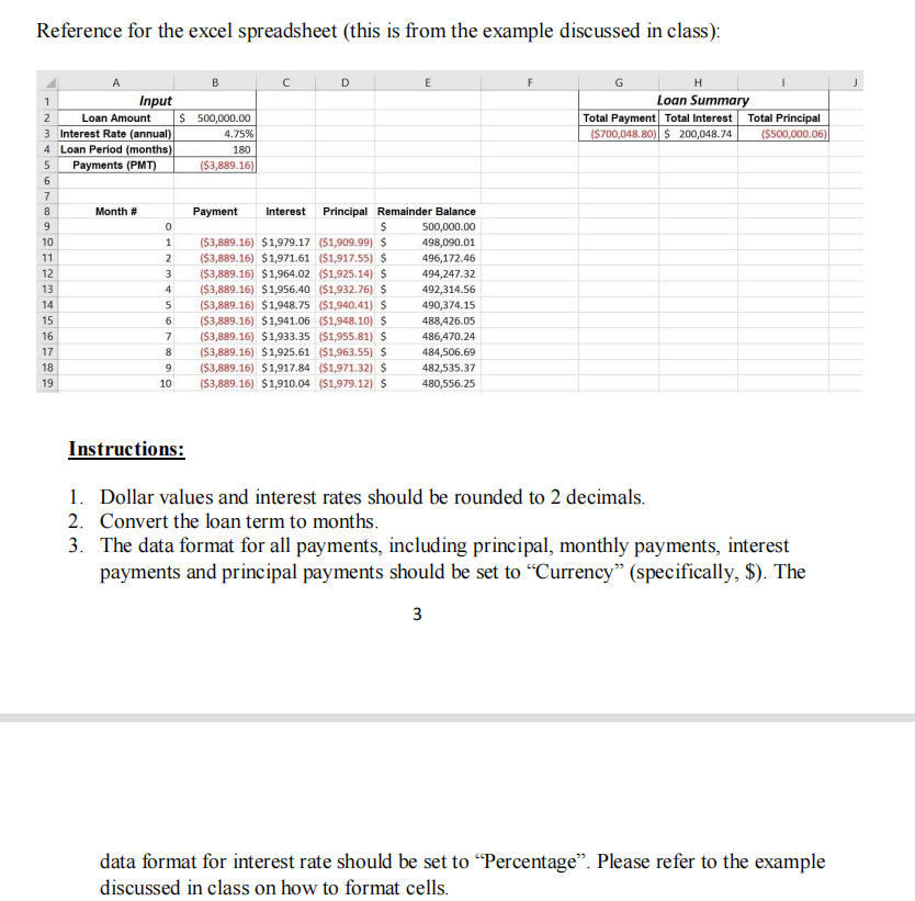
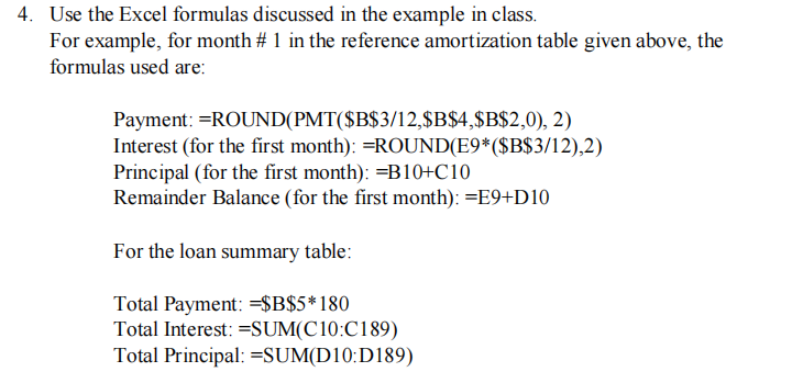
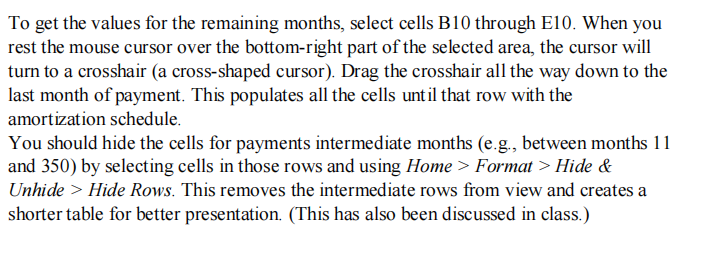
Reference for the excel spreadsheet (this is from the example discussed in class): B C D G Input Loan Summary Loan Amount 500,000.00 Total Payment


Step by Step Solution
There are 3 Steps involved in it
Step: 1

Get Instant Access to Expert-Tailored Solutions
See step-by-step solutions with expert insights and AI powered tools for academic success
Step: 2

Step: 3
Ace Your Homework with AI
Get the answers you need in no time with our AI-driven, step-by-step assistance
Get Started
Research Design Qualitative Quantitative And Mixed Methods Approaches
Authors: John W. Creswell, J. David Creswell
5th Edition
1506386709, 9781506386706