Reporting Adjusted Account Balances

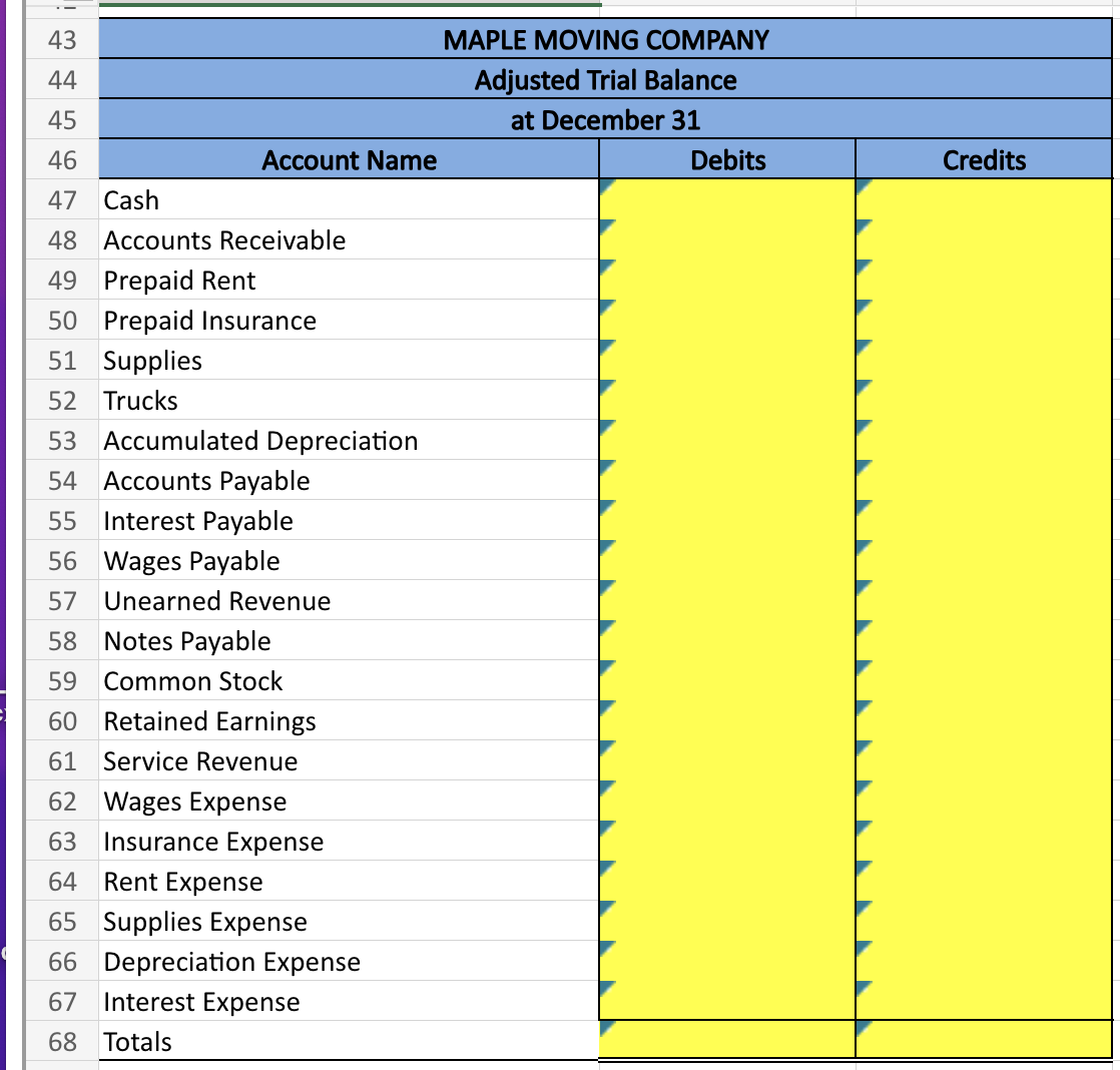
Maple Moving Company has provided you with their unadjusted balances before year-end adjustments. The Controller has asked you to prepare the Adjusted Trial Balance and has provided you with further year-end information.

Cash-$62,000

Accounts Receivable- $51,000

Prepaid Rent-$1,000

Prepaid Insurance-$750

Supplies- $67,600

Trucks- $176,000

Accumulated Depreciation-17,600

Accounts Payable-$37,500

Interest Payable-$5,000

Wages Payable-$ 10,000

Unearned Revenue-$6,600

Notes Payable-$100,000

Common Stock-$66,000

Retained Earnings-$23,400

Service Revenue-$167,000

Wages Expense-$61,000

Insurance Expense- 61,000

Rent Expense- 11,000

Supplies Expense- 0

Depreciation Expense- 0

Interest Expense-0

Required: Use the above account balances and the following year-end data to determine adjusted account balances and prepare an adjusted trial balance.

One month of rent used: $1,000

One month of insurance used: $250

Interest owed but not paid yet: $10,800

Supplies on hand: $15,000

Truck depreciation expense: $35,200

Unpaid wages earned by employees: $3,500

Unearned revenue that has been earned: $2,000

** Please provide answers to the above image, in the form of (example) =B4+B5 for the cell reference or "= =SUM(C7,C8,C9) to the side of the answer for further clarification.

Basic Math Functions: Allows you to use the basic math symbols to perform mathematical functions. You can use the following keys: + (plus sign to add), - (minus sign to subtract), *(asterisk to multiply), and / (forward slash to divide). For example, if you entered '=B4+B5" in a blank cell, the formula would add the values from those cells and output the result.

SUM Function: Allows you to refer to multiple cells and add all the values. You can add individual cell references or ranges. If you entered =SUM(C4,C5,C6) into a blank cell, the formula would output the result of adding those three separate cells. Similarly, if you entered =SUM(C4:C6), the formula would output the same result of adding those cells.

\begin{tabular}{ll|l|l|} \hline 43 & \multicolumn{2}{|c|}{ MAPLE MOVING COMPANY } \\ \hline 44 & \multicolumn{1}{|c|}{ Adjusted Trial Balance } \\ \hline 45 & \multicolumn{1}{|c|}{ Account Name } & \\ \hline 46 & \multicolumn{1}{|c|}{ December 31 } \\ \hline 47 & Cash & \\ \hline 48 & Accounts Receivable & \\ \hline 50 & Prepaid Rent & \\ \hline 51 & Supplies & \\ \hline 52 & Trucks & \\ \hline 53 & Accumulated Depreciation & \\ \hline 54 & Accounts Payable & \\ \hline 55 & Interest Payable & \\ \hline 56 & Wages Payable & \\ \hline 57 & Unearned Revenue & \\ \hline 58 & Notes Payable & \\ \hline 59 & Common Stock & \\ \hline 60 & Retained Earnings & \\ \hline 61 & Service Revenue & \\ \hline 62 & Wages Expense & \\ \hline 63 & Insurance Expense & \\ \hline 64 & Rent Expense & \\ \hline 65 & Supplies Expense & \\ \hline 66 & Depreciation Expense & \\ \hline 67 & Interest Expense & \\ \hline 68 & Totals & \\ \hline \end{tabular}