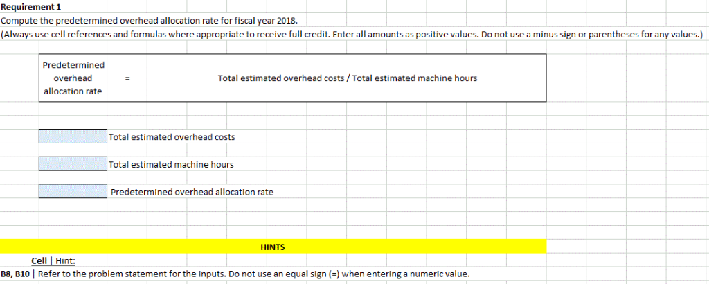
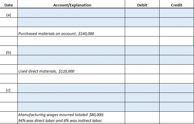
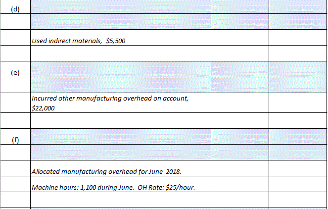
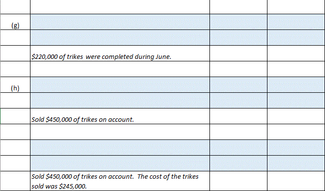
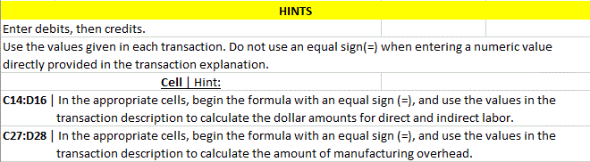
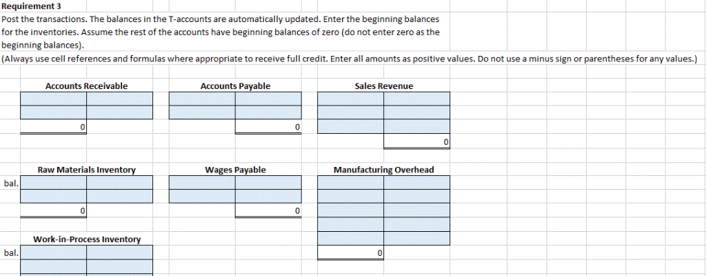
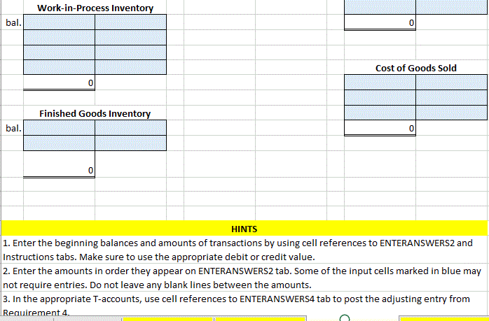
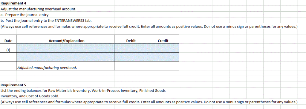
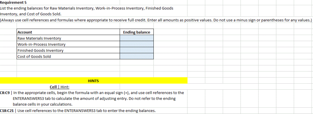
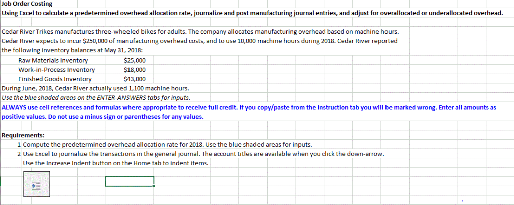
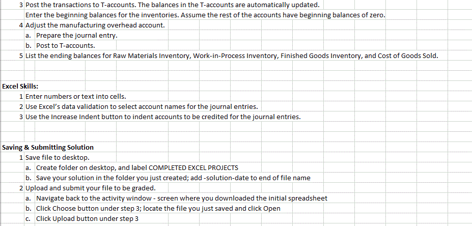
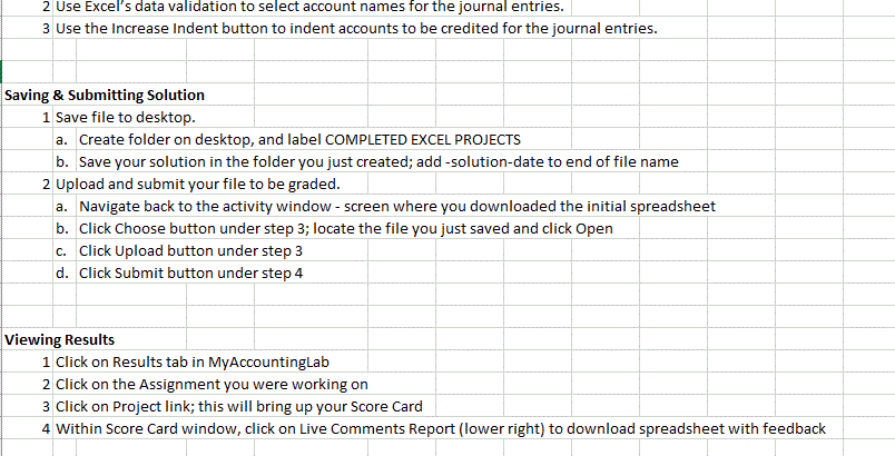
Requirement 1 Compute the predetermined overhead allocation rate for fiscal year 2018. s positive values. Do not use a minus sign or parentheses for any values.) (Always use cell references and formulas where appropriate to receive full credit. Enter all amounts Predetermined overhead Total estimated overhead costs/Total estimated machine hours allocation rate Total estimated overhead costs Total estimated machine hours Predetermined overhead allocation rate HINTS Cell Hint B8, B10 Refer to the problem statement for the inputs. Do not use an equal sign ()when entering a numeric value. Requirement 2 Journalize the transactions in the general journal. (Scroll down to view hints.) (Always use formulas where appropriate to receive full credit. Enter all amounts as positive values. Do not use a minus sign or parentheses for any values.) Account/Explanation Debit Credit Date Purchased materials on account, $140,000 (b) Used direct materials, $110,000 (c) Manufacturing wages incurred totaled $80,000; 94% was direct labor and 6% was indirect labor (d) Used indirect materials, $5,500 (e) Incurred other manufacturing overhead on account, $22,000 (f) Allocated manufacturing overhead for June 2018. Machine hours: 1,100 during June. OH Rate: $25/hour 17 (g) $220,000 of trikes were completed during June. (h) Sold $450,000 of trikes on account Sold $450,000 of trikes on account. The cost of the trikes sold was $245,000. HINTS Enter debits, then credits Use the values given in each transaction. Do not use an equal sign() when entering a numeric value directly provided in the transaction explanation Cell Hint C14:D16 In the appropriate cells, begin the formula with an equal sign (, and use the values in the transaction description to calculate the dollar amounts for direct and indirect labor. C27:D28 | In the appropriate cells, begin the formula with an equal sign (), and use the values in the transaction description to calculate the amount of manufacturing overhead. Requirement 3 Post the transactions. The balances in the T-accounts are automatically updated. Enter the beginning balances for the inventories. Assume the rest of the accounts have beginning balances of zero (do not enter zero as the beginning balances). (Always use cell references and formulas where appropriate to receive full credit. Enter all amounts as positive values. Do not use a minus sign or parentheses for any values.) Accounts Payable Accounts Receivable Sales Revenue 0 Wages Payable Raw Materials Inventory Manufacturing Overhead bal. 0 0 Work-in-Process Inventory bal. Work-in-Process Inventory bal Cost of Goods Sold 0 Finished Goods Inventory bal. 0 0 HINTS 1. Enter the beginning balances and amounts of transactions by using cell references to ENTERANSWERS2 and Instructions tabs. Make sure to use the appropriate debit or credit value. 2. Enter the amounts in order they appear on ENTERANSWERS2 tab. Some of the input cells marked in blue may not require entries. Do not leave any blank lines between the amounts. 3. In the appropriate T-accounts, use cell references to ENTERANSWERS4 tab to post the adjusting entry from Requirement 4. Requirement 4 Adjust the manufacturing overhead account. a. Prepare the journal entry. b. Post the journal entry to the ENTERANSWERS3 tab. (Always use cell references and formulas where appropriate to receive full credit. Enter all amounts as positive values. Do not use a minus sign or parentheses for any values.) Account/Explanation Debit Credit Date i) Adjusted manufacturing overhead. Requirement 5 List the ending balances for Raw Materials Inventory, Work-in-Process Inventory, Finished Goods Inventory, and Cost of Goods Sold. (Always use cell references and formulas where appropriate to receive full credit. Enter all amounts as positive values. Do not use a minus sign or parentheses for any values.) Requirement 5 List the ending balances for Raw Materials Inventory, Work-in- Process Inventory, Finished Goods nventory, and Cost of Goods Sold. Always use cell references and formulas where appropriate to receive full credit. Enter all amounts as positive values. Do not use a minus sign or parentheses for any values.) Account Ending balance Raw Materials Inventory Work-in-Process Inventory Finished Goods Inventory Cost of Goods Sold HINTS Cell Hint: C8:C9 In the appropriate cells, begin the formula with an equal sign (), and use cell references to the ENTERANSWERS3 tab to calculate the amount of adjusting entry. Do not refer to the ending balance cells in your calculations. C18:C21 | Use cell references to the ENTERANSWERS3 tab to enter the ending balances. Job Order Costing Using Excel to calculate a predetermined overhead allocation rate, journalize and post manufacturing journal entries, and adjust for overallocated or underallocated overhead. Cedar River Trikes manufactures three-wheeled bikes for adults. The company allocates manufacturing overhead based on machine hours. Cedar River expects to incur $250,000 of manufacturing overhead costs, and to use 10,000 machine hours during 2018. Cedar River reported the following inventory balances at May 31, 2018: Raw Materials Inventory $25.000 $18,000 Work-in-Process Inventory Finished Goods Inventory During June, 2018, Cedar River actually used 1,100 machine hours Use the blue shaded areas on the ENTER-ANSWERS tabs for inputs. ALWAYS use cell references and formulas where appropriate to receive full credit. If you copy/paste from the Instruction tab you will be marked wrong. Enter all amounts as $43,000 positive values. Do not use a minus sign or parentheses for any values. Requirements: 1 Compute the predetermined overhead allocation rate for 2018. Use the blue shaded areas for inputs 2 Use Excel to journalize the transactions in the general journal. The account titles are available when you click the down-arrow. Use the Increase Indent button on the Home tab to indent items. 3 Post the transactions to T-accounts. The balances in the T-accounts are automatically updated. Enter the beginning balances for the inventories. Assume the rest of the accounts have beginning balances of zero. |Adjust the manufacturing overhead account. 4 a. Prepare the journal entry. b. Post to T-accounts. 5 List the ending balances for Raw Materials Inventory, Work-in-Process Inventory, Finished Goods Inventory, and Cost of Goods Sold. Excel Skills: 1 Enter numbers or text into cells. 2 Use Excel's data validation to select account names for the journal entries. 3 Use the Increase Indent button to indent accounts to be credited for the journal entries. Saving & Submitting Solution 1 Save file to desktop a. Create folder on desktop, and label COMPLETED EXCEL PROJECTS b. Save your solution in the folder you just created; add -solution-date to end of file name 2 Upload and submit your file to be graded. a. Navigate back to the activity window - screen where you downloaded the initial spreadsheet b. Click Choose button under step 3; locate the file you just saved and click Open C. Click Upload button under step 3 2 Use Excel's data validation to select account names for the journal entries. 3 Use the Increase Indent button to indent accounts to be credited for the journal entries. Saving & Submitting Solution 1 Save file to desktop a. Create folder on desktop, and label COMPLETED EXCEL PROJECTS b. Save your solution in the folder you just created; add -solution-date to end of file name 2 Upload and submit your file to be graded. Navigate back to the activity window - screen where you downloaded the initial spreadsheet a. b. Click Choose button under step 3; locate the file you just saved and click Open c. Click Upload button under step 3 d. Click Submit button under step 4 Viewing Results 1 Click on Results tab in MyAccountingLab 2 Click on the Assignment you were working on V 3 Click on Project link; this will bring up your Score Card 4 Within Score Card window, click on Live Comments Report (lower right) to download spreadsheet with feedback Requirement 1 Compute the predetermined overhead allocation rate for fiscal year 2018. s positive values. Do not use a minus sign or parentheses for any values.) (Always use cell references and formulas where appropriate to receive full credit. Enter all amounts Predetermined overhead Total estimated overhead costs/Total estimated machine hours allocation rate Total estimated overhead costs Total estimated machine hours Predetermined overhead allocation rate HINTS Cell Hint B8, B10 Refer to the problem statement for the inputs. Do not use an equal sign ()when entering a numeric value. Requirement 2 Journalize the transactions in the general journal. (Scroll down to view hints.) (Always use formulas where appropriate to receive full credit. Enter all amounts as positive values. Do not use a minus sign or parentheses for any values.) Account/Explanation Debit Credit Date Purchased materials on account, $140,000 (b) Used direct materials, $110,000 (c) Manufacturing wages incurred totaled $80,000; 94% was direct labor and 6% was indirect labor (d) Used indirect materials, $5,500 (e) Incurred other manufacturing overhead on account, $22,000 (f) Allocated manufacturing overhead for June 2018. Machine hours: 1,100 during June. OH Rate: $25/hour 17 (g) $220,000 of trikes were completed during June. (h) Sold $450,000 of trikes on account Sold $450,000 of trikes on account. The cost of the trikes sold was $245,000. HINTS Enter debits, then credits Use the values given in each transaction. Do not use an equal sign() when entering a numeric value directly provided in the transaction explanation Cell Hint C14:D16 In the appropriate cells, begin the formula with an equal sign (, and use the values in the transaction description to calculate the dollar amounts for direct and indirect labor. C27:D28 | In the appropriate cells, begin the formula with an equal sign (), and use the values in the transaction description to calculate the amount of manufacturing overhead. Requirement 3 Post the transactions. The balances in the T-accounts are automatically updated. Enter the beginning balances for the inventories. Assume the rest of the accounts have beginning balances of zero (do not enter zero as the beginning balances). (Always use cell references and formulas where appropriate to receive full credit. Enter all amounts as positive values. Do not use a minus sign or parentheses for any values.) Accounts Payable Accounts Receivable Sales Revenue 0 Wages Payable Raw Materials Inventory Manufacturing Overhead bal. 0 0 Work-in-Process Inventory bal. Work-in-Process Inventory bal Cost of Goods Sold 0 Finished Goods Inventory bal. 0 0 HINTS 1. Enter the beginning balances and amounts of transactions by using cell references to ENTERANSWERS2 and Instructions tabs. Make sure to use the appropriate debit or credit value. 2. Enter the amounts in order they appear on ENTERANSWERS2 tab. Some of the input cells marked in blue may not require entries. Do not leave any blank lines between the amounts. 3. In the appropriate T-accounts, use cell references to ENTERANSWERS4 tab to post the adjusting entry from Requirement 4. Requirement 4 Adjust the manufacturing overhead account. a. Prepare the journal entry. b. Post the journal entry to the ENTERANSWERS3 tab. (Always use cell references and formulas where appropriate to receive full credit. Enter all amounts as positive values. Do not use a minus sign or parentheses for any values.) Account/Explanation Debit Credit Date i) Adjusted manufacturing overhead. Requirement 5 List the ending balances for Raw Materials Inventory, Work-in-Process Inventory, Finished Goods Inventory, and Cost of Goods Sold. (Always use cell references and formulas where appropriate to receive full credit. Enter all amounts as positive values. Do not use a minus sign or parentheses for any values.) Requirement 5 List the ending balances for Raw Materials Inventory, Work-in- Process Inventory, Finished Goods nventory, and Cost of Goods Sold. Always use cell references and formulas where appropriate to receive full credit. Enter all amounts as positive values. Do not use a minus sign or parentheses for any values.) Account Ending balance Raw Materials Inventory Work-in-Process Inventory Finished Goods Inventory Cost of Goods Sold HINTS Cell Hint: C8:C9 In the appropriate cells, begin the formula with an equal sign (), and use cell references to the ENTERANSWERS3 tab to calculate the amount of adjusting entry. Do not refer to the ending balance cells in your calculations. C18:C21 | Use cell references to the ENTERANSWERS3 tab to enter the ending balances. Job Order Costing Using Excel to calculate a predetermined overhead allocation rate, journalize and post manufacturing journal entries, and adjust for overallocated or underallocated overhead. Cedar River Trikes manufactures three-wheeled bikes for adults. The company allocates manufacturing overhead based on machine hours. Cedar River expects to incur $250,000 of manufacturing overhead costs, and to use 10,000 machine hours during 2018. Cedar River reported the following inventory balances at May 31, 2018: Raw Materials Inventory $25.000 $18,000 Work-in-Process Inventory Finished Goods Inventory During June, 2018, Cedar River actually used 1,100 machine hours Use the blue shaded areas on the ENTER-ANSWERS tabs for inputs. ALWAYS use cell references and formulas where appropriate to receive full credit. If you copy/paste from the Instruction tab you will be marked wrong. Enter all amounts as $43,000 positive values. Do not use a minus sign or parentheses for any values. Requirements: 1 Compute the predetermined overhead allocation rate for 2018. Use the blue shaded areas for inputs 2 Use Excel to journalize the transactions in the general journal. The account titles are available when you click the down-arrow. Use the Increase Indent button on the Home tab to indent items. 3 Post the transactions to T-accounts. The balances in the T-accounts are automatically updated. Enter the beginning balances for the inventories. Assume the rest of the accounts have beginning balances of zero. |Adjust the manufacturing overhead account. 4 a. Prepare the journal entry. b. Post to T-accounts. 5 List the ending balances for Raw Materials Inventory, Work-in-Process Inventory, Finished Goods Inventory, and Cost of Goods Sold. Excel Skills: 1 Enter numbers or text into cells. 2 Use Excel's data validation to select account names for the journal entries. 3 Use the Increase Indent button to indent accounts to be credited for the journal entries. Saving & Submitting Solution 1 Save file to desktop a. Create folder on desktop, and label COMPLETED EXCEL PROJECTS b. Save your solution in the folder you just created; add -solution-date to end of file name 2 Upload and submit your file to be graded. a. Navigate back to the activity window - screen where you downloaded the initial spreadsheet b. Click Choose button under step 3; locate the file you just saved and click Open C. Click Upload button under step 3 2 Use Excel's data validation to select account names for the journal entries. 3 Use the Increase Indent button to indent accounts to be credited for the journal entries. Saving & Submitting Solution 1 Save file to desktop a. Create folder on desktop, and label COMPLETED EXCEL PROJECTS b. Save your solution in the folder you just created; add -solution-date to end of file name 2 Upload and submit your file to be graded. Navigate back to the activity window - screen where you downloaded the initial spreadsheet a. b. Click Choose button under step 3; locate the file you just saved and click Open c. Click Upload button under step 3 d. Click Submit button under step 4 Viewing Results 1 Click on Results tab in MyAccountingLab 2 Click on the Assignment you were working on V 3 Click on Project link; this will bring up your Score Card 4 Within Score Card window, click on Live Comments Report (lower right) to download spreadsheet with feedback