Scenario Pastas R Us, Inc. is a fast-casual restaurant chain specializing in noodle-based dishes, soups, and salads. Since its inception, the business development team has favored opening new restaurants in areas (within a 3-mile radius) that satisfy the following demographic conditions: ? Median age between 25 and 45 years old ? Household median income above national average ? At least 15% college-educated adult population Last year, the marketing department rolled out a loyalty card strategy to increase sales. Under this program, customers present their loyalty card when paying for their orders and receive some free food after making 10 purchases. The company has collected data from its 74 restaurants to track important variables such as average sales per customer, year-on-year sales growth, sales per sq. ft., loyalty card usage as a percentage of sales, and others. A key metric of financial performance in the restaurant industry is annual sales per sq. ft. For example, if a 1,200 sq. ft. restaurant recorded $2 million in sales last year, then it sold $1,667 per sq. ft. Executive management wants to know whether the current expansion criteria can be improved; evaluate the effectiveness of the loyalty card marketing strategy; and identify feasible, actionable opportunities for improvement. As a member of the analytics department, you've been assigned the responsibility of conducting a thorough statistical analysis of the company's available database to answer executive management's questions.

I have already completed this portion.

Part 1: Descriptive Statistics Analysis Conduct the following descriptive statistics analyses using the Pastas R Us, Inc. data set in Microsoft Excel. Answer the questions in the spreadsheet or a separate Microsoft Word document. Insert a new column in the database that corresponds to AnnualSales. AnnualSales is the result of multiplying a restaurant's

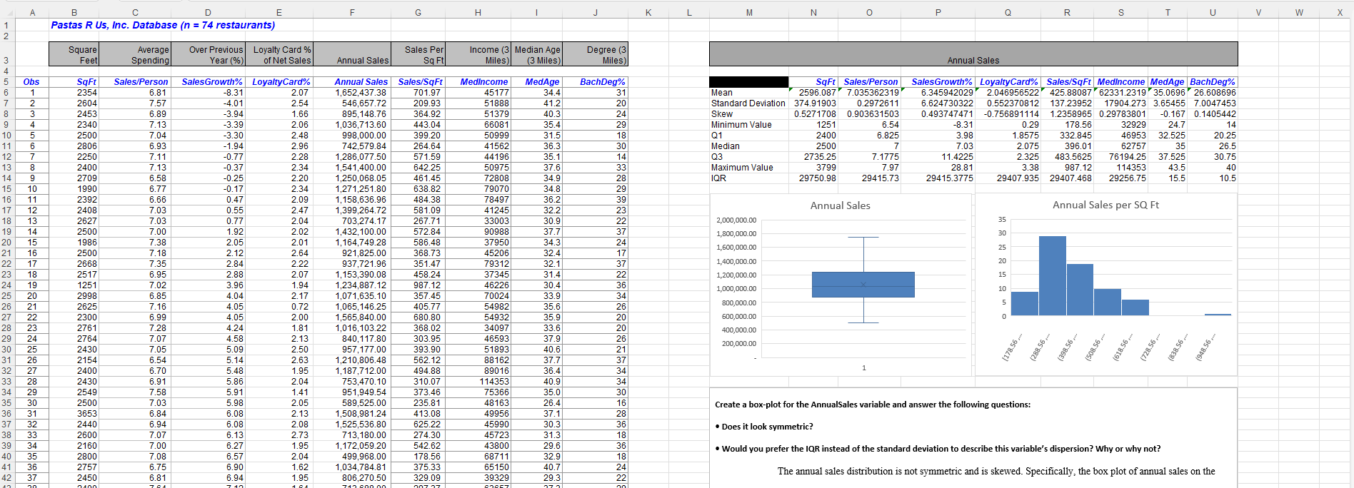
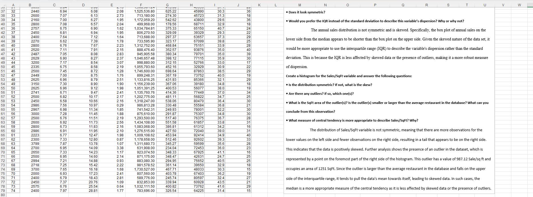
SqFt by Sales/SqFt. Calculate the following: ? mean ? standard deviation ? skew ? 5-number summary ? interquartile range (IQR) for each of the variables box-plot for the AnnualSales variable and answer the following questions: ? Does it look symmetric? ? Would you prefer the IQR instead of the standard deviation to describe this variable's dispersion? Why or why not? histogram for the Sales/SqFt variable and answer the following questions: ? Is the distribution symmetric? If not, what is the skew? ? Are there any outliers? If so, which one(s)? ? What is the SqFt area of the outlier(s)? Is the outlier(s) smaller or larger than the average restaurant in the database? What can you conclude from this observation? ? What measure of central tendency is more appropriate to describe Sales/SqFt? Why? I have already completed this portion.

B C D E F G H K M N 0 P Q R S T U V W Pastas R Us, Inc. Database (n = 74 restaurants) Square Average Over Previous Loyalty Card % Sales Per Income (3| Median Age Degree (3 Feet Spending Year (%) of Net Sales Annual Sales Sq Ft Miles) (3 Miles) Miles) Annual Sales AW obs SqFt Sales/Person SalesGrowth% LoyaltyCard% Annual Sales Sales/SqFt Medincome MedAge BachDeg SqFt Sales/Person SalesGrowth% LoyaltyCard% Sales/SqFt Medincome MedAge BachDeg% 2354 6.81 8.31 2.07 1,652,437.38 701.97 45177 34.4 31 Mean 2596.087 7.035362319 6.345942029 2.046956522 425.88087 62331.2319 35.0696 26.608696 2604 7.57 4.01 2.54 546,657.72 209.93 1888 41.2 20 Standard Deviation 374.91903 0.2972611 6.624730322 0.552370812 137.23952 17904.273 3.65455 7.0047453 8 2453 6.89 -3.94 1.66 895, 148.76 364.92 51379 40.3 24 Skew 0.5271708 0.903631503 0.493747471 -0.756891114 1.2358965 0.29783801 -0.167 0.1405442 9 2340 7.13 -3.39 2.06 1,036,713.60 443.04 66081 35.4 29 Minimum Value 1251 6.54 -8.31 0.29 178.56 32929 24.7 14 10 2500 7.04 -3.30 2.48 998,000.00 399.20 50999 31.5 18 Q1 2400 6.825 3.98 1.8575 832.845 46953 32.525 20.25 11 2806 6.93 -1.94 2.96 742,579.84 264.64 41562 36.3 30 Median 2500 7.03 2.075 396.01 62757 35 26.5 12 2250 7.11 -0.77 2.28 1,286,077.50 571.59 44196 35.1 14 Q3 2735.25 7.1775 1.4225 2.325 483.5625 76194.25 37.525 30.75 13 2400 7.13 -0.37 2.34 1,541,400.0 642.25 50975 37.6 33 Maximum Value 3799 7.97 28.81 3.38 987.12 114353 43.5 40 14 2709 6.58 -0.25 2.20 1,250,068.05 461.45 72808 34.9 28 IQR 29750.98 29415.73 29415.3775 29407.935 29407.468 29256.75 15.5 10.5 15 10 1990 6.77 -0.17 2.34 1,271,251.80 638.82 79070 34.8 29 16 11 2392 6.66 0.47 2.09 1,158,636.96 484.38 78497 36.2 39 17 12 2408 7.03 0.55 2.47 1,399,264.72 581.09 41245 32.2 23 Annual Sales Annual Sales per SQ Ft 18 13 2627 7.03 0.77 2.04 703,274.17 267.71 33003 30.9 22 2,000,000.00 19 14 2500 7.00 1.92 2.02 1,432, 100.00 572.84 90988 37.7 37 1,800,000.00 20 15 1986 7.38 2.05 2.01 1,164,749.28 586.48 37950 34.3 24 21 16 2500 7.18 2.12 2.64 921,825.00 368.73 45206 32.4 17 1,600,000.00 17 2668 7.35 2.84 2.22 937,721.96 351.47 79312 32.1 37 1,400,000.00 18 2517 6.95 2.88 2.07 1,153,390.08 458.24 37345 31.4 22 1,200,000.00 1251 7.02 3.96 1.94 1,234,887.12 987.12 46226 30. 4 36 1,000,000.00 2998 6.85 4.04 2.17 1,071,635.10 357.45 70024 3.9 34 2625 7.16 4.05 0.72 1,065, 146.25 405.77 54982 35.6 26 800,000.00 2300 6.99 4.05 2.00 1,565,840.00 680.80 54932 35.9 20 600,000.00 28 2761 7.28 4.24 1.81 1,016, 103.22 368.02 34097 33.6 20 400,000.00 29 2764 7.07 4.58 2.13 840, 117.80 303.95 46593 37.9 26 30 2430 7.05 5.09 2.50 957,177.00 393.90 51893 40.6 21 200,000.00 [178.56 ,. (288.56 ,.. (398.56 ,.. (508.56 ,.. (618.56 ,. (728.56 ,.. (838.56 ,.. (948.56 ,.. 2154 6.54 5.14 2.63 1,210,806.48 562.12 88162 37.7 37 2400 6.70 5.48 1.95 1,187,712.00 494.88 89016 36.4 34 2430 6.91 5.86 2.04 753,470.10 310.07 14353 40.9 34 29 2549 7.58 5.91 1.41 951,949.54 373.46 75366 35.0 30 30 2500 7.03 5.98 2.05 589,525.00 235.81 4816 26.4 16 Create a box-plot for the AnnualSales variable and answer the following questions: 3653 6.84 6.08 2.13 1,508,981.24 413.08 19956 37.1 28 2440 6.94 6.08 2.08 1,525,536.80 625.22 45990 30.3 36 . Does it look symmetric? 2600 7.07 6.13 2.73 713, 180.00 274.30 45723 31.3 18 3286848 2160 7.00 6.27 1.95 , 172,059.20 542.62 43800 29.6 36 32.9 . Would you prefer the IQR instead of the standard deviation to describe this variable's dispersion? Why or why not? 2800 7.08 6.57 2.04 499,968.00 178.56 68711 18 2757 6.75 6.90 1.62 1,034,784.81 375.33 55150 40.7 24 2450 6.81 6.94 1.95 806,270.50 9329 29.3 The annual sales distribution is not symmetric and is skewed. Specifically, the box plot of annual sales on thea7 38 39 40 a 42 43 44 45 46 47 48 49 50 51 52 53 54 55 56 57 58 59 60 61 62 63 64 65 66 67 68 69 70 7 72 73 74 75 76 77 78 79 80 2440 2600 2160 2800 2757 2450 2400 2270 2800 2520 2487 2629 3200 2335 2500 2449 2625 2150 2625 211 2500 2450 2986 2967 2000 2500 2600 2800 2986 2223 2300 2799 2700 2650 2500 2994 2718 3700 2000 2400 2450 2575 2400 6.94 7.07 7.00 7.08 6.75 6.81 7.64 6.62 6.76 71 7.05 6.90 77 6.75 7.45 7.00 6.96 7.20 6.96 671 6.82 6.58 7.56 6.98 728 6.76 6.92 6.73 6.91 677 733 7.87 6.95 7.33 6.95 7.21 725 7.65 6.93 6.79 7.37 6.76 797 6.08 6.13 6.27 6.57 6.90 6.94 712 7.39 7.67 7.91 8.08 8.27 8.54 8.58 8.72 8.75 8.79 8.90 9.12 9.47 1017 10.66 10.97 1134 11.45 11.51 11.73 11.83 11.95 12.47 12.80 1378 14.09 14.23 14.60 14.88 15.42 16.18 17.23 18.43 20.76 25.54. 28.81 208 273 1.95 204 162 195 164 178 223 215 2383 237 3.07 219 128 176 251 190 1.98 241 217 218 029 1.85 188 219 256 216 210 1.08 087 107 338 147 214 093 222 1.68 241 281 1.09 064 177 F 1,525,536.80 713,180.00 1,172,059.20 409,968.00 1,034,784.81 806,270.50 713,688.00 733,595.90 1,312,752.00 888,476.40 945,905.58 1,046,657.48 998,830.00 1,085,793.60 1,746,600.00 899,248.31 1,133,816.25 1,156,239.00 1,051,391.25 1,135,760.76 1,202,775.00 1,318,247.00 986,813.28 74154231 875,610.00 1,293,500.00 1,434,108.00 1,083,068.00 1,276,515.00 1,009,108 62 1,178,656.00 1,311,680.73 631,908.00 923,074.50 871,175.00 883,080.30 981,578.52 1,730,527.00 807,560.00 589,776.00 832,853.00 1,032,11150 783,696.00 e 62522 45990 303 36 27430 45723 313 18 54262 43800 295 36 17856 68711 329 18 37533 65150 407 24 320.09 30329 203 22 297.37 63657 373 29 32317 67099 398 25 46884 75151 338 28 35257 93876 35.0 40 380.34 79701 35.0 39 398.12 77115 359 30 312.15 52766 330 17 45216 32929 308 22 698.64 87863 385 29 367.19 73752 405 19 43193 85366 321 29 367.08 20180 34.8 18 40053 56077 380 19 41436 77449 37.0 34 48111 56822 347 25 538.06 80470 364, 30 330.48 55584 368 21 249.93 78001 322 30 20187 75307 34.8 30 517.40 76375 367 28 55158 61857 338 31 386.81 61312 342 16 42750 72040 39.0 31 45304 92414 349 40 512.46 92602 393 33 34527 59599 35.6 28 23404 72453 36.0 23 34833 67925 411 16 348.47 42631 247 25 29495 75652 405 25 361.14 30650 329 18 467.71 48033 303 15 40378 67403 362 19 24574 80597 324, 27 339.94 60928 435 21 400.82 73762 416 29 32654 64225 314, 15 " N o P a R s T u v w Does it look symmetric? * Would you prefer the IQR instead of the standard deviation to describe this variable's dispersion? Why or why not? 'The annual sales distribution is not symmetric and is skewed. Specifically, the box plot of annual sales on the Tower side from the median appears to be shorter than the box plot on the upper side. Given the skewed nature of the data set, it would be more appropriate to use the interquartile range (IQR) to describe the variable's dispersion rather than the standard deviation. This is because the IQR is less affected by skewed data or the presence of outliers, making it 2 more robust measure of dispersion Create a histogram for the Sales/SaFt vari le and answer the following questio Is the distribution symmetric? If not, what is the skew? * Are there any outliers? If so, which one(s)? * What is the SqFt area of the outlier{s]? Is the outlier(s) smaller or larger than the average restaurant in the database? What can you conclude from this observation? + What measure of central tendency is more appropriate to describe Sales/SqFt? Why? The distribution of Sales/SqFt variable is not symmetric, meaning that there are more observations for the lower values on the left side and fewer observations on the right side, resulting in a tail that appears to be on the right side. This indicates that the data is positively skewed. Further analysis shows the presence of an outlier in the dataset, which is resented by a point on the foremost part of the right side of the histogram. This outlier has a value of 987.12 Sale/sq ft and occupies an area of 1251 SqFt. Since the outlier is larger than the average restaurant in the database and falls on the upper side of the interquartile range, it tends to pull the data's mean towards itself, leading to skewed data. In such cases, the median is a more appropriate measure of the central tendency as it is less affected by skewed data or the presance of outliers