Scenario Question

In March 2010, McDonald's Corp. announced a policy to increase summer sales by selling all soft drinks, no matter the size, for $1.00. The policy would run for 150 days starting after Memorial Day. The $1.00 drink prices were a discount from the suggested price of $1.39 for a large soda. Some franchisees worried that discounting drinks, whose sales compensate for discounts on other products, could hurt overall profits, especially if customers bought other items from the Dollar Menu. McDonald's managers expected this promotion would draw customers from other fast-food chains and from convenience stores such as 7-Eleven. Additional customers would also help McDonald's push its new beverage lineup that included smoothies and frappes. Discounted drinks did cut into McDonald's coffee sales in previous years as some customers chose the drinks rather than pricier espresso beverages. Other chains with new drink offerings, such as Burger King and Taco Bell, could face pressure from the $1.00 drinks at McDonald's

Question:

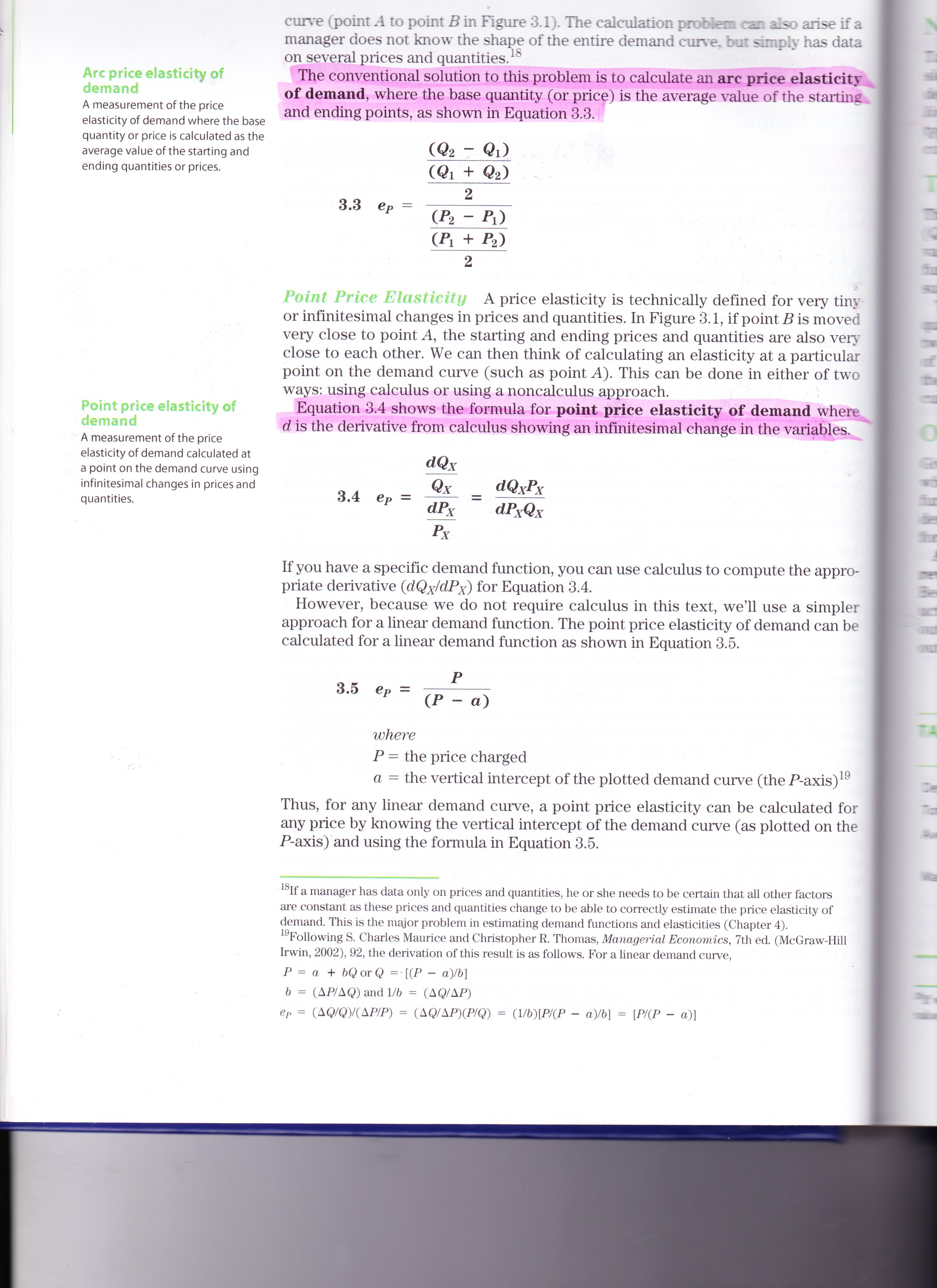
a.) Given the change in price for a large soda from $1.39 to $1.00, how much would quantity demanded have to increase for McDonald's revenues to increase? ( Use the arc elasticity formula for any percentage change calculations.)

b.) What is the sign of the implied cross-price elasticity with drinks from McDonald's competitors?

c.) What are the other benefits and costs to McDonald's of this discount drink policy?

These are the formulas: arc elasticity formula (Top)

point price elasticity (Bottom)

curve (point A to point B in Figure 3.1). The calculation problem can also arise if a manager does not know the shape of the entire demand curve, but simply has data on several prices and quantities. 18 Arc price elasticity of The conventional solution to this problem is to calculate an arc price elasticity demand of demand, where the base quantity (or price) is the average value of the starting A measurement of the price elasticity of demand where the and ending points, as shown in Equation 3.3. quantity or price is calculated as the average value of the starting and ( Q 2 - Q1 ) ending quantities or prices. ( Q 1 + @ 2 ) 2 3.3 ep = (P2 - P1) (P1 + P2) Point Price Elasticity A price elasticity is technically defined for very tiny or infinitesimal changes in prices and quantities. In Figure 3.1, if point B is moved very close to point A, the starting and ending prices and quantities are also very close to each other. We can then think of calculating an elasticity at a particular point on the demand curve (such as point A). This can be done in either of two ways: using calculus or using a noncalculus approach. Point price elasticity of Equation 3.4 shows the formula for point price elasticity of demand where demand d is the derivative from calculus showing an infinitesimal change in the variables. A measurement of the price elasticity of demand calculated at a point on the demand curve using dQx infinitesimal changes in prices and dQxPx quantities. 3.4 ep = Qx dP x = dP xQx Px If you have a specific demand function, you can use calculus to compute the appro- priate derivative (dQx/dPx) for Equation 3.4. However, because we do not require calculus in this text, we'll use a simpler approach for a linear demand function. The point price elasticity of demand can be calculated for a linear demand function as shown in Equation 3.5. 3.5 ep = ( P - where P = the price charged a = the vertical intercept of the plotted demand curve (the P-axis) 19 Thus, for any linear demand curve, a point price elasticity can be calculated for any price by knowing the vertical intercept of the demand curve (as plotted on the P-axis) and using the formula in Equation 3.5. 18If a manager has data only on prices and quantities, he or she needs to be certain that all other factors are constant as these prices and quantities change to be able to correctly estimate the price elasticity of demand. This is the major problem in estimating demand functions and elasticities (Chapter 4). Following S. Charles Maurice and Christopher R. Thomas, Managerial Economics, 7th ed. (McGraw-Hill Irwin, 2002), 92, the derivation of this result is as follows. For a linear demand curve, P = a + bQ or Q = [(P - a)/b] b = (AP/AQ) and 1/b = (AQ/AP) ep = (AQIQ)/(AP/P) = (AQIAP)(PIQ) = (1/b)[P/(P - a)/b] = [P/(P - a)]