show answer with formula please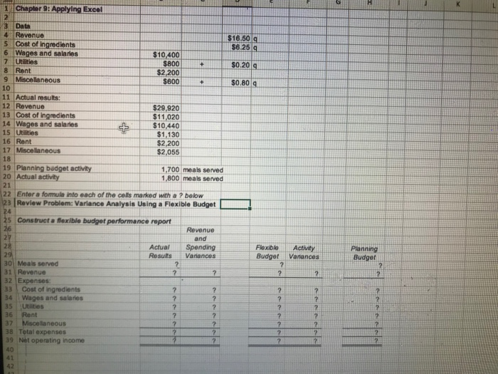

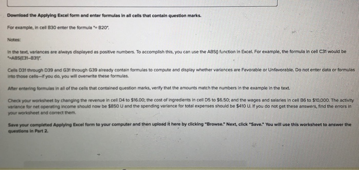
G H Chapter 9: Applying Excel $16.50 9 $6 25 7 $0.20 + $0.80 9 Data Revenue Cost of ingredients 6 Wages and salaries $10,400 Utilities $800 + 8 Rent $2,200 9 Miscellaneous $600 10 11 Actual results: 12 Revenue $29,920 13 Cost of Ingredients $11,020 14 Wages and salaries + $10,440 15 Utilities $1,130 16 Rent $2,200 17 Miscellaneous $2,055 18 19 Planning budget activity 1.700 meals served 20 Actual activity 1,800 meals served 21 22 Enter a formule into each of the colls marked with a ? below 23 Review Problem: Variance Analysis Using a Flexible Budget 24 25 Construct a flexible budget performance report 26 Revenue 27 and 28 Actual Spending 29 Results Varances 30 Meals served 2 31 Revenue ? ? 32 Expenses 33 Cost of ingredients ? 34 Wages and salaries 35 Utilities ? ? 36 Rent ? ? 37 Miscellaneous ? ? 38 Total expenses ? ? 39 Net operating income ? 40 Flexible Budget 2 ? Activity Vanances Planning Budger 2 2 2 2 2 2 ? ? 2 2 2 ? ? 7 2 ? 2 ? ? 2 ? ? ? ? 2 2 42 Download the Applying Excel form and enter formulas in all cells that contain question marks. For example, in cell 830 enter the formule - B20". Notes: In the text, variances are always displayed as posilve numbers. To accomplish this, you can use the ABSQ function in Excel. For example, the formula in cel c31 would be *ABS(E31-3311. Cells 031 through D39 and G31 through G39 already contain formulas to compute and display whether variances are Favorable or Unfavorable. Do not enter cata or formulas Into those cels- you do, you will overwrite these formulas. After entering formulas in all of the cells that contained question marks, verify that the amounts match the numbers in the example in the text. Check your worksheet by changing the revenue in cell D4 to $16.00; the cost of ingredients in cell D5 to $6.50; and the wages and solaries in cell 86 to $10,000. The activity variance for net operating income should now be $850 U and the spending variance for total expenses should be $410 U. If you do not get these answers, find the errors in your worksheet and correct them. Save your completed Applying Excel form to your computer and then upload it here by clicking "Browse."Next, click Save. You will use this worksheet to answer the questions in Part 2