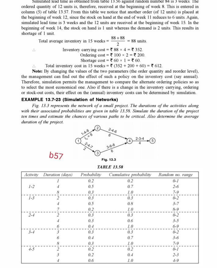
Simulated lead time as obtained from table 13.56 against random number 84 is 3 weeks. The ordered quantity of 12 units is, therefore, received at the beginning of week 8. This is entered in column (5) of table 13.57. From this table we notice that another order (of 12 units) is placed at the beginning of week 12, since the stock on hand at the end of week 11 reduces to 6 units. Again, simulated lead time is 3 weeks and the 12 units are received at the beginning of week 15. In the beginning of week 14, the stock on hand is 1 unit whereas the demand is 2 units. This results in shortage of 1 unit 88 + 88 Total average inventory in 15 weeks = 88 units. 2 Inventory carrying cost = * 88 4 = * 352 Ordering cost = 100 x 2 = 200. Shortage cost * 60 * 1 = 60 Total inventory cost in 15 weeks = ? (352 + 200 + 60) = 3612. Note: By changing the values of the two parameters (the order quantity and reorder level), the management can find out the effect of such a policy on the inventory cost (say annual). Therefore, simulation permits the management to compare the alternate ordering policies so as to select the most economical one. Also if there is a change in the inventory carrying, ordering or stock-out costs, their effect on the annual) inventory costs can be determined by simulation EXAMPLE 13.7-23 (Simulation of Networks) Fig. 13.3 represents the network of a small project. The durations of the activities along with their associated probabilities are given in table 13.58. Simulate the duration of the project ten times and estimate the chances of various paths to be critical. Also determine the average duration of the project. 2-4-6 1-4-8 8 6 lo 2-3-4 2-4-7 2 3-6-8 6 b57 Activity Duration (days) 1 1-2 4 0-1 1-3 Fig. 13.3 TABLE 13.58 Probability Cumulative probability Random no. range 0.2 0.2 0.5 0.7 2-6 0.3 1.0 7-9 0.3 0.3 0-2 0.5 0.8 3-7 0.2 1.0 8-9 0.3 0.3 0-2 0.3 0.6 3-5 0.4 1.0 6-9 0.3 0.3 0-2 0.4 0.7 3-6 0.3 1.0 7-9 0.2 0.2 2-3 0.6 1.0 4-9 2-4 W 3-4 a la NICO 4-5 2 3 0.2 0.4